11 Full telemetry

As well as the sparse, low frequency telemetry that we can capture from the live data service whilst a stage is running, more substantial telemetry datasets are published several hours after a stage has run when the WRC onboard video views are made available.

The density of points is high enough to allow us to make a reasonable estimate on how far a car is into to the stage based simply on summing the distances between consecutive sample locations. However, this does mean that the distance metric is dependent on the actual route taken by a driver. Whilst drivers will typically take a similar line, a more exact comparison based on distance into the stage can be generated by mapping each sample location on the nearest location on the official route.

Inspection of the telemetry files suggests that the data is presented in a common form, with actual clock start represented by a negative time stamp injected into the second row of the dataframe. (The first and third rows are perhaps actual telemetry data.)

Load in the full resolution telemetry:

get_full_telem = function (fp, proj=utm_proj4_string, utm=FALSE){
  # TO DO - the proj parameter is not used?
  telem_df_full_raw = read.csv(fp)  %>% drop_na("lon", "lat") %>% 
                  map_df(rev) %>%
   # Omit the negative start time in row 2
   filter(utx > 0)  %>%
   mutate(utc = as_datetime(utx/1000))

  # We could further tune the locations to be projections onto the route
  # This would then ensure a normalisation of the distance into the stage
  # against a common origin
  
  # TO DO - here we explicitly set the lat long crs
  # TO DO - don't use the literal 4326
  telem_df_full_raw$lonX = telem_df_full_raw$lon
  telem_df_full_raw$latX = telem_df_full_raw$lat
  telem_df_full = telem_df_full_raw  %>%
                    st_as_sf(coords = c("lonX","latX")) %>% st_set_crs(4326)

  # Inject name from file name into dataframe
  # Remove accents
  clean_fp = stringi::stri_trans_general(fp, "Latin-ASCII")
  metadata = str_match(fp, ".*df_telemetrymergeddata_(SS.*)_(.*).csv")
  stage_ =  metadata[2]
  driver_ = str_trim(stringi::stri_trans_general(metadata[3], "Latin-ASCII"))
  
  telem_df_full$driver = driver_
  telem_df_full$stage = stage_
  
  # If required, we can get a UTM projection at this point
  if (utm) {
     telem_df_full_utm =  st_transform(telem_df_full,
                           crs = st_crs(utm_proj4_string))
     telem_df_full_utm
  } else {
    telem_df_full
  }
}

We can then load the telemetry data in

fn="df_telemetrymergeddata_SS7_Evans.csv"
telem_df_full = get_full_telem(file.path(path, fn))

How many data points?

nrow(telem_df_full %>% st_coordinates() ) 

## [1] 4377

As we can see, the full telemetry gives us quite closely sampled points along the route:

leaflet(telem_df_full) %>% 
  addProviderTiles("OpenTopoMap", group = "OSM") %>% 
  addCircleMarkers(weight = 1)

Or how about plotting the data using ggplot:

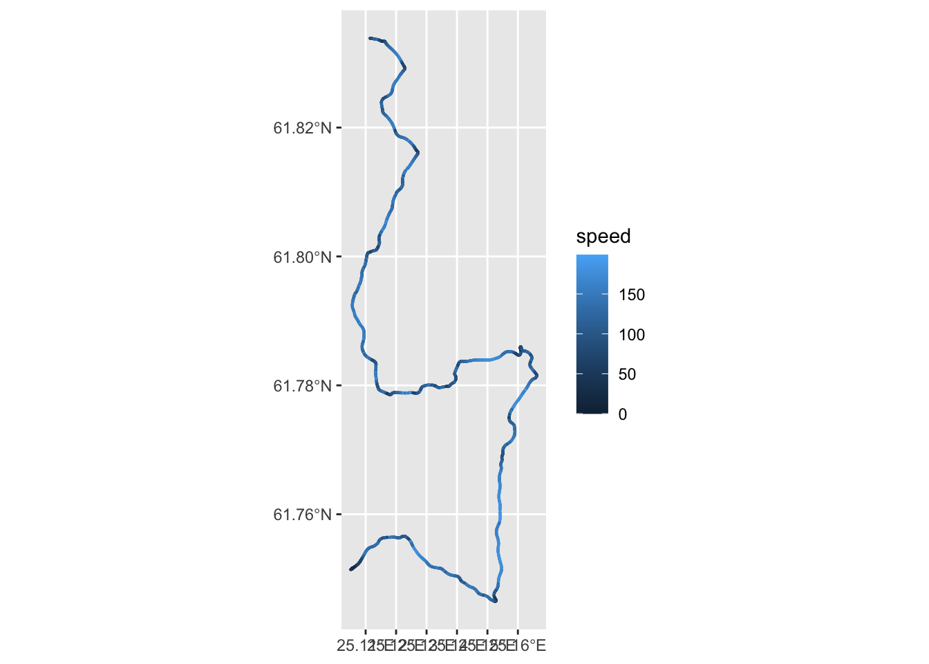
ggplot(data=telem_df_full) + geom_sf(aes(color=speed), size=0.1)