5 Plotting Locations a Certain Time Into the Stage

In order to calculate the time into stage, we need to set the time series origin somehow. If we have a telemetry data point recorded at the start stage start (location wise) when the light goes green, we can use that time as the time origin. But what if that data is not available, which is highly likely when working with low resolution live location data?

5.1 Find the Stage Telemetry Time Series Origin

One approach would be to look to the timing and results data for data describing the start time of the stage for the particular data. This time can then be used as the tie origin (with a check to make sure it looks sensible!). But this approach brings with it the overhead of having to lookup that data via the WRC API.

We can also set the time from a time passed as a string. For example:

explicit_time_origin = ymd_hms("2020-04-01 10:30:13", tz=timezone)

5.1.1 Estimating the Start Time

If we are missing timing data from the start of the run, and we assume that the run started exactly on the minute, we can round down the first sample time to get to the next nearest minute using the lubridate::round_date() function:

first_time = route_telem_utm[1,]$utc

first_time_rounded = round_date(first_time, unit="1 minutes")

c(first_time, first_time_rounded)

## [1] "2021-10-02 08:37:23 UTC" "2021-10-02 08:37:00 UTC"

We can then use the rounded first time as a basis for a running stage time estimate by subtracting that time from the sample datetimes:

# Get stage time as a time object...
route_telem_utm$roundeddelta_t = route_telem_utm$utc - first_time_rounded
# And in seconds
route_telem_utm$roundeddelta_s = as.double(route_telem_utm$roundeddelta_t)

X	driverid	heading	kms	name	speed	status	track	utx	X_rally_stageid	X_carentryid	X_telemetryID	X_name	delta	utc	geometry	dist	roundeddelta_t	roundeddelta_s
1870	NA	144	0.6	33	166	Competing	NA	1.633164e+12	bcc5537d-d28a-40af-ba86-95dad7fb9cd1	b185c5df-8115-40cf-bd81-566f016f6bf5	/a3f5f3f5-3fb0-42ab-af90-24d91c0493d0/ss07eva_telemetry_js/js	Evans	0	2021-10-02 08:37:23	POINT (401052.2 6856758)	531.9830	23.6 secs	23.6
1869	NA	150	0.7	33	140	Competing	NA	1.633164e+12	bcc5537d-d28a-40af-ba86-95dad7fb9cd1	b185c5df-8115-40cf-bd81-566f016f6bf5	/a3f5f3f5-3fb0-42ab-af90-24d91c0493d0/ss07eva_telemetry_js/js	Evans	3200	2021-10-02 08:37:26	POINT (401117.6 6856633)	673.7129	26.8 secs	26.8
1868	NA	172	0.8	33	60	Competing	NA	1.633164e+12	bcc5537d-d28a-40af-ba86-95dad7fb9cd1	b185c5df-8115-40cf-bd81-566f016f6bf5	/a3f5f3f5-3fb0-42ab-af90-24d91c0493d0/ss07eva_telemetry_js/js	Evans	6400	2021-10-02 08:37:30	POINT (401142.7 6856572)	746.9263	30.0 secs	30.0
1867	NA	220	0.9	33	107	Competing	NA	1.633164e+12	bcc5537d-d28a-40af-ba86-95dad7fb9cd1	b185c5df-8115-40cf-bd81-566f016f6bf5	/a3f5f3f5-3fb0-42ab-af90-24d91c0493d0/ss07eva_telemetry_js/js	Evans	9600	2021-10-02 08:37:33	POINT (401093 6856511)	825.5652	33.2 secs	33.2
1866	NA	210	1.0	33	149	Competing	NA	1.633164e+12	bcc5537d-d28a-40af-ba86-95dad7fb9cd1	b185c5df-8115-40cf-bd81-566f016f6bf5	/a3f5f3f5-3fb0-42ab-af90-24d91c0493d0/ss07eva_telemetry_js/js	Evans	12800	2021-10-02 08:37:36	POINT (401020.1 6856413)	947.9104	36.4 secs	36.4
1865	NA	208	1.1	33	159	Competing	NA	1.633164e+12	bcc5537d-d28a-40af-ba86-95dad7fb9cd1	b185c5df-8115-40cf-bd81-566f016f6bf5	/a3f5f3f5-3fb0-42ab-af90-24d91c0493d0/ss07eva_telemetry_js/js	Evans	16000	2021-10-02 08:37:39	POINT (400938.8 6856299)	1088.1680	39.6 secs	39.6

5.1.2 Using a False Origin

Another approach to setting the origin is to not set one; or rather, to start the time series with a false origin, such as the first location point. The time into stage (from the false origin) can then be found by using the sample time of the first in-stage telemetry data point as the time origin set at that location.

false_origin_time = route_telem_utm$utc[1]
false_origin_time

## [1] "2021-10-02 08:37:23 UTC"

And then generate deltas from that:

# Get stage time as a time object...
route_telem_utm$falsedelta_t = route_telem_utm$utc - false_origin_time
# And in seconds
route_telem_utm$falsedelta_s = as.double(route_telem_utm$falsedelta_t)

kable(head(route_telem_utm %>% select(c(utc, roundeddelta_t, roundeddelta_s,
                                        falsedelta_t, falsedelta_s))),
      format = "html") %>%
  kable_styling() %>%
  kableExtra::scroll_box(width = "100%")

utc	roundeddelta_t	roundeddelta_s	falsedelta_t	falsedelta_s	geometry
2021-10-02 08:37:23	23.6 secs	23.6	0.0 secs	0.0	POINT (401052.2 6856758)
2021-10-02 08:37:26	26.8 secs	26.8	3.2 secs	3.2	POINT (401117.6 6856633)
2021-10-02 08:37:30	30.0 secs	30.0	6.4 secs	6.4	POINT (401142.7 6856572)
2021-10-02 08:37:33	33.2 secs	33.2	9.6 secs	9.6	POINT (401093 6856511)
2021-10-02 08:37:36	36.4 secs	36.4	12.8 secs	12.8	POINT (401020.1 6856413)
2021-10-02 08:37:39	39.6 secs	39.6	16.0 secs	16.0	POINT (400938.8 6856299)

This approach might also extended for use when comparing two or more drivers, by setting a false origin for each driver, then rebasing against a common origin set at the location origin furthest into the start for the drivers being compared.

5.2 Plotting the Stage Telemetry Time Series

We can now plot the distance into stage and the stage time (as per the telemetry sample points) relative to each other.

ggplot(route_telem_utm) +geom_line(aes(x=dist, y=roundeddelta_s))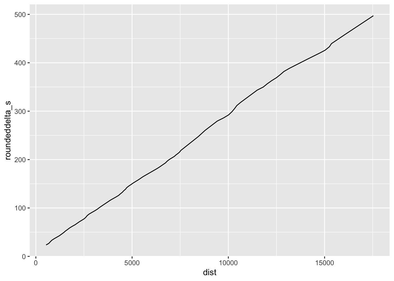

If we have data for two or more cars, this would start to provide a basis for comparison. For example, we might be able to see the distance along the stage where their times diverge.

We might also plot a distance versus time graph.