14 Looking At Braking Behaviour

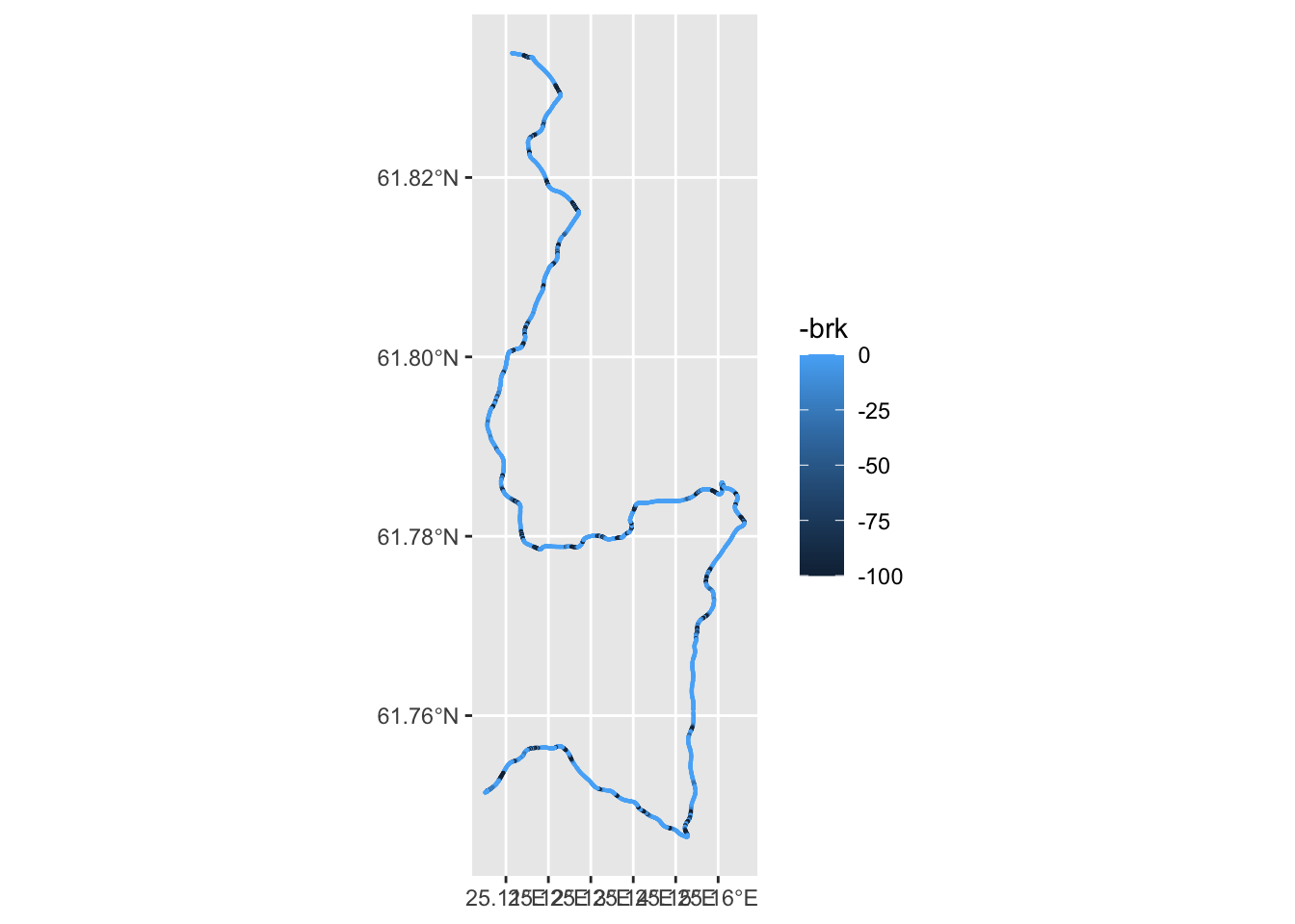
Where do we brake?

#library(ggspatial)
#  annotation_spatial(trj_ogier ) +
#  layer_spatial(trj_ogier, aes(alpha = brk), color='red',size=0.3) 

#https://github.com/eliocamp/ggnewscale
# Multiple color scales
# ?doesn't work with geom_sf which overplots?
library(ggnewscale)

## Warning: package 'ggnewscale' was built under R version 4.0.5

ggplot() + stat_sf_coordinates(aes( color=throttle),size=0.1,
  geom = "point",
 data=trj_ogier %>% filter(throttle>0)) +
scale_color_gradient(low = "white", high = "green") +
 new_scale_color() + 
scale_color_gradient(low = "white", high = "red")+ stat_sf_coordinates( aes( color=brk), size=0.1,
  geom = "point",
  data=trj_ogier %>% filter(brk>0)
) + 
# How do we get the correct projection
#_coord_map()
# Already rectilinear...
  coord_fixed()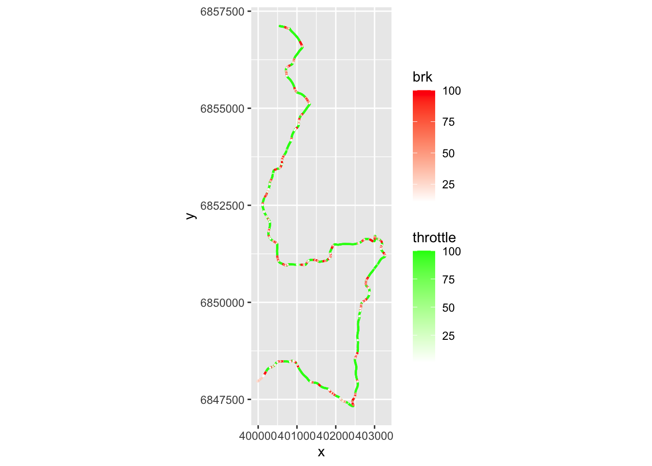

14.1 Throttle Comparison

How do our two drivers compare in their use of the throttle?

ggplot() +
  geom_line(data=(trj_ogier %>% filter(cum_dist>=1000 & cum_dist<=2000)),
            aes(x=cum_dist,y=throttle), color='red') +
  geom_line(data=(trj_evans %>% filter(cum_dist>=1000 & cum_dist<=2000)),
            aes(x=cum_dist,y=throttle), color='blue')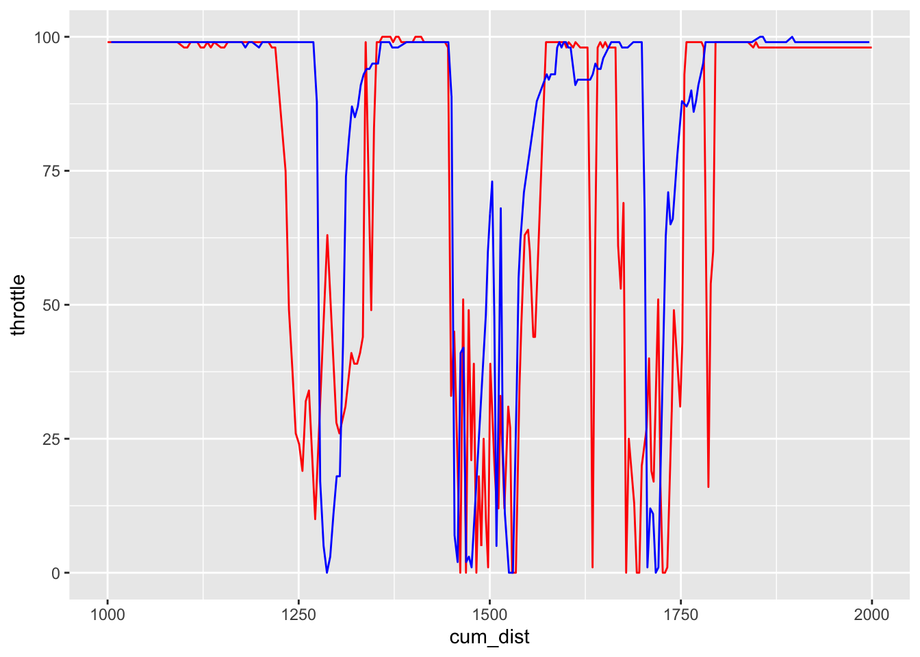

With smoothing:

library(zoo)

## 
## Attaching package: 'zoo'

## The following objects are masked from 'package:base':
## 
##     as.Date, as.Date.numeric

ggplot() +
  geom_line(data=trj_ogier%>% filter(cum_dist>=1000 & cum_dist<=2000) %>%
                    mutate(smooth_throttle=rollmean(throttle, k = 3, fill = NA)),
            aes(x=cum_dist,y=smooth_throttle), color='red') +
  geom_line(data=(trj_evans %>% filter(cum_dist>=1000 & cum_dist<=2000) %>%
                    mutate(smooth_throttle=rollmean(throttle, k = 3, fill = NA))),
            aes(x=cum_dist,y=smooth_throttle), color='blue')

## Warning: Removed 2 row(s) containing missing values (geom_path).
## Removed 2 row(s) containing missing values (geom_path).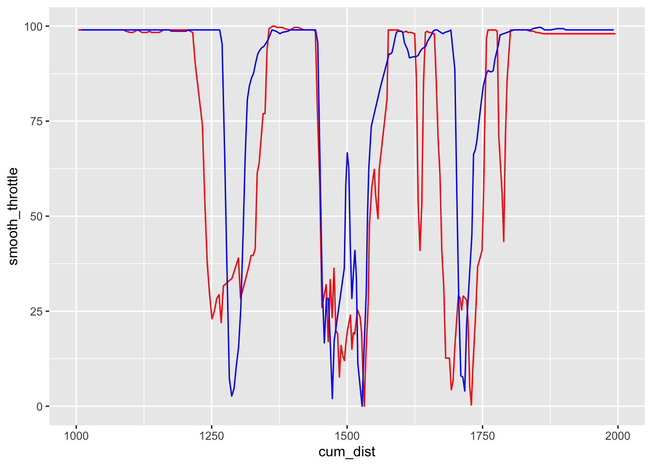

We can also explore adding throttle and brake data to the speed trace.

theme_black = function(base_size = 12, base_family = "") {
  
  theme_grey(base_size = base_size, base_family = base_family) %+replace%
    
    theme(
      # Specify axis options
      axis.line = element_blank(),  
      axis.text.x = element_text(size = base_size*0.8, color = "white", lineheight = 0.9),  
      axis.text.y = element_text(size = base_size*0.8, color = "white", lineheight = 0.9),  
      axis.ticks = element_line(color = "white", size  =  0.2),  
      axis.title.x = element_text(size = base_size, color = "white", margin = margin(0, 10, 0, 0)),  
      axis.title.y = element_text(size = base_size, color = "white", angle = 90, margin = margin(0, 10, 0, 0)),  
      axis.ticks.length = unit(0.3, "lines"),   
      # Specify legend options
      legend.background = element_rect(color = NA, fill = "black"),  
      legend.key = element_rect(color = "white",  fill = "black"),  
      legend.key.size = unit(1.2, "lines"),  
      legend.key.height = NULL,  
      legend.key.width = NULL,      
      legend.text = element_text(size = base_size*0.8, color = "white"),  
      legend.title = element_text(size = base_size*0.8, face = "bold", hjust = 0, color = "white"),  
      legend.position = "right",  
      legend.text.align = NULL,  
      legend.title.align = NULL,  
      legend.direction = "vertical",  
      legend.box = NULL, 
      # Specify panel options
      panel.background = element_rect(fill = "black", color  =  NA),  
      panel.border = element_rect(fill = NA, color = "white"),  
      panel.grid.major = element_line(color = "grey35"),  
      panel.grid.minor = element_line(color = "grey20"),  
      panel.margin = unit(0.5, "lines"),   
      # Specify faceting options
      strip.background = element_rect(fill = "grey30", color = "grey10"),  
      strip.text.x = element_text(size = base_size*0.8, color = "white"),  
      strip.text.y = element_text(size = base_size*0.8, color = "white",angle = -90),  
      # Specify plot options
      plot.background = element_rect(color = "black", fill = "black"),  
      plot.title = element_text(size = base_size*1.2, color = "white"),  
      plot.margin = unit(rep(1, 4), "lines")
      
    )
  
}

What happens if we try to colour the speed line according to the throttle and brake percentages?

ggplot() +
  #geom_line(data=trj_ogier %>% filter(cum_dist>=1000 & cum_dist<=2000),
  #          aes(x=cum_dist,y=speed), color='white', size=4) +
   geom_line(data=trj_ogier %>% filter(cum_dist>=1000 & cum_dist<=2000),
            aes(x=cum_dist,y=speed, alpha=throttle), size=1, color="green") +
  geom_line(data=trj_ogier %>% filter(cum_dist>=1000 & cum_dist<=2000),
            aes(x=cum_dist,y=speed-3, alpha=brk), color="red", size=1) +
   geom_line(data=trj_ogier %>% filter(cum_dist>=1000 & cum_dist<=2000),
            aes(x=cum_dist,y=throttle-50, alpha=100-brk), size=1, color="green") +
  geom_line(data=trj_ogier %>% filter(cum_dist>=1000 & cum_dist<=2000),
            aes(x=cum_dist,y=brk-50, alpha=100-throttle), color="red", size=1)+
  
  theme_black()+ theme(legend.position="none")

## Warning: `panel.margin` is deprecated. Please use `panel.spacing` property
## instead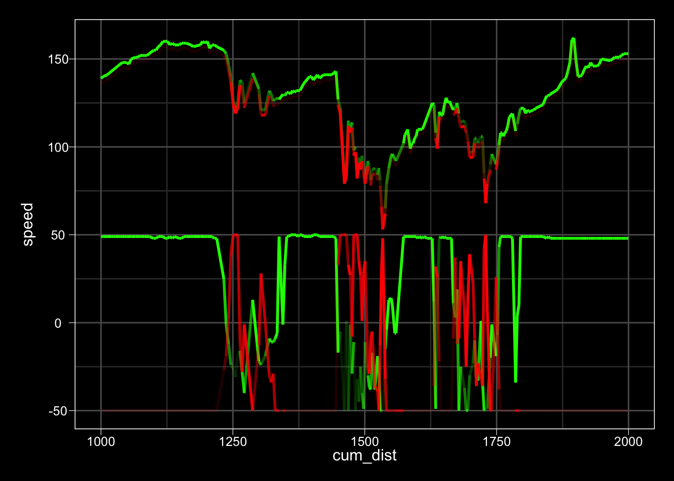

ggplot(data=telem_df_full) + geom_sf(aes(color=throttle), size=0.1)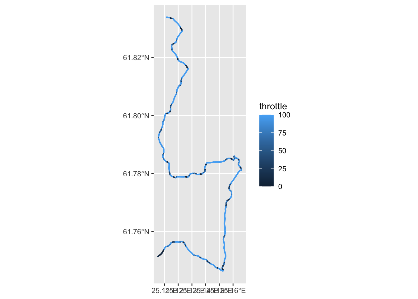

ggplot(data=telem_df_full) + geom_sf(aes(color=-brk), size=0.1)