7 Accessing and Working With Elevation Data Raster Files
Having access to the stage route data allows us to render its shape using a recognisable map projection using tools such as ggplot2(). We can also display a route in an interactive map overlaid over familiar map tiles using leaflet.
Being able to plot the route on a simple 2D map gives us a good sense of how twisty and turny a route may be, and plotting it on a terrain themed tileset gives us an impression of how the elevation may vary along the route. But can we do better than that, by getting actual elevation data?
7.1 Introducing Digital Elevation Model (DEM) Raster Images
In recent decades, international efforts have combined to produce a wide range of openly licensed and freely available topographic datasets that contain elevation data spanning the globe. Known as digital elevation models (DEM), the data is often published using two dimensional raster images that can be indexed and retrieved in a similar way to map tiles but where colour channels within separate image layers may used to encode elevation values, as well as other data sets.
In this chapter, we will review various ways of obtaining and downloading elevation raster data, as well as some simple ways of previewing it.
In particular, we will introduce two different techniques for downloading elevation data for specified geographical areas:
- using the
elevatrR package to download data ; - using the
geoviz::mapzen()R package to download image data via Mapzen.
7.1.1 What Is Raster Data?
A raster or raster image is a pixel based representation in which each pixel represents an area on the Earth’s surface. Many popular file formats, including JPEG, PNG and TIFF image formats, as well as more specialised forms.
The spatial resolution of the image describes the surface covered by each pixel, from coarse grained resolutions of 1km square or more to finer resolutions at the 50-100m level to detailed imaging at the sub-1 meter square level.
The extent of the raster describes the geographical extent covered by the image. A coordinate reference system (CRS) string describes the co-ordinate system and geographical projection that identifies how a grid based co-ordinate system overlaid on a globe model of the Earth is “projected” onto a two dimensional map based view of the world.
7.1.2 What Are Digital Elevation Models (DEMs)?
Digital Elevation Models (DEM), also known as digital terrain models (DTM), are digital models that encode the elevation of the area on the Earth’s surface they correspond to. DEMS seek to represent the elevation of the Earths surface level, rather than the elevation of surface features such as buildings or trees, which tend to be described using digital surface models. DEMs are typically represented using image raster files where pixel values encode elevation values rather than visual features.
Further reading:
- [GIS Wiki: Digital Elevation Model] (http://wiki.gis.com/wiki/index.php/Digital_Elevation_Model)
- Introduction to Geographic Information Systems, R. Adam Dastrup, 6.2: Raster Data Models*
- Essentials of Geographic Information Systems, Campbell and Shin, 4.1: Raster Data Models
- For a review of raster image file formats, see Raster data file format lists in GIS
- For sources of openly available DEM data, see for example [Mapzen terrain data sources ](https://github.com/tilezen/joerd/blob/master/docs/data-sources.md
7.1.3 The R raster Package
The R raster package provides a wide range of tools for opening, viewing, manipulating and saving raster images.
For a good introduction to raster image data in general, and working with raster images in R in particular, see the National Ecological Observatory Network (NEON) tutorial on Raster Data in R - The Basics.
For working with distance calculations over rasters, see the geodist R package.
7.2 Downloading Elevation Data
Requesting data from an elevation data service requires us to provide the area for which we want to retrieve the elevation data in terms of an identifying location and an extent.
We can look-up the latitude and longitude co-ordinates and general extent of each stage route from the stage route file, so let’s start by loading in some sample stage data.
Elevation data is published by a wide variety of sources with national and international scope. National datasets are often at a higher spatial resolution (smaller grid size on the ground)
7.2.1 Loading in some stage data
We can load in some example stage data from a geojson file we have downloaded previously:
# Load in the tidyr package to provide various utilities, such as %>%
library(tidyr)

# Load in the stage data from a geojson file
geojson_filename = 'montecarlo_2021.geojson'
geojson_sf = sf::st_read(geojson_filename)
## Reading layer `montecarlo_2021' from data source `/Users/tonyhirst/Documents/GitHub/visualising-rally-stages/montecarlo_2021.geojson' using driver `GeoJSON'
## Simple feature collection with 9 features and 2 fields
## geometry type: LINESTRING
## dimension: XY
## bbox: xmin: 5.243488 ymin: 43.87633 xmax: 6.951953 ymax: 44.81973
## geographic CRS: WGS 84From the loaded in simple features object, we can access the bounding box encompassing all the stages in the rally or the bounding box from a selected stage or stages:
# Obtain the bounding box around the first stage
stage_bbox = sf::st_bbox(geojson_sf[1,])
7.2.2 Obtaining relief / elevation raster data using elevatr
The elevatr package allows us to retrieve elevation rasters from various sources, including the Amazon Web Services Terrain Tiles, the Open Topography Global Datasets API, and the USGS Elevation Point Query Service.
The raster::get_elev_raster() functions downloads DEMs as a raster image covering one or more locations, the extent of sp or sf data object, and a zoom level.
Note that when passing sf or sp objects, a projection that uses meters is required.
If we are in the latlong projection with units of degrees, we can create a simple dataframe containing the locations of the bounding box co-ordinates:
ex.df <- data.frame(x= c(stage_bbox[['xmin']], stage_bbox[['xmax']]),
                    y= c(stage_bbox[['ymin']], stage_bbox[['ymax']]))
ex.df
## x y
## 1 5.883753 44.73562
## 2 5.940715 44.81973and then pass that to the elevatr::get_elev_raster() function:
library(raster)
library(elevatr)

# The zoom level, z, impacts on how long it takes to download the imagery
# z ranges from 1 to 14
# https://www.rdocumentation.org/packages/elevatr/versions/0.3.4/topics/get_elev_raster
prj_dd <- "+proj=longlat +ellps=WGS84 +datum=WGS84 +no_defs"
elev_img <- get_elev_raster(ex.df, prj = prj_dd, z = 12, clip = "bbox")
#elev_img <- get_elev_raster(as(geojson_sf[1,],'Spatial'), z = 12, clip = "bbox")
elev_img
## class : RasterLayer
## dimensions : 565, 382, 215830 (nrow, ncol, ncell)
## resolution : 0.0001488281, 0.0001488281 (x, y)
## extent : 5.883827, 5.94068, 44.73566, 44.81975 (xmin, xmax, ymin, ymax)
## crs : +proj=longlat +datum=WGS84 +no_defs
## source : memory
## names : file6d535c9607cf
## values : 663, 2055 (min, max)We can preview the raster image by plotting it:
raster::plot(elev_img)
7.2.3 Plotting Rasters As ggplot Objects
Using the rasterVis::gplot() function, we can render an a raster image as a ggplot2 object:
library(rasterVis)

gr = gplot(elev_img) +
        geom_tile(aes(fill = value)) +
        scale_fill_gradientn(colours = rev(terrain.colors(225))) +
        coord_equal() + theme_void() + theme(legend.position = "none")

gr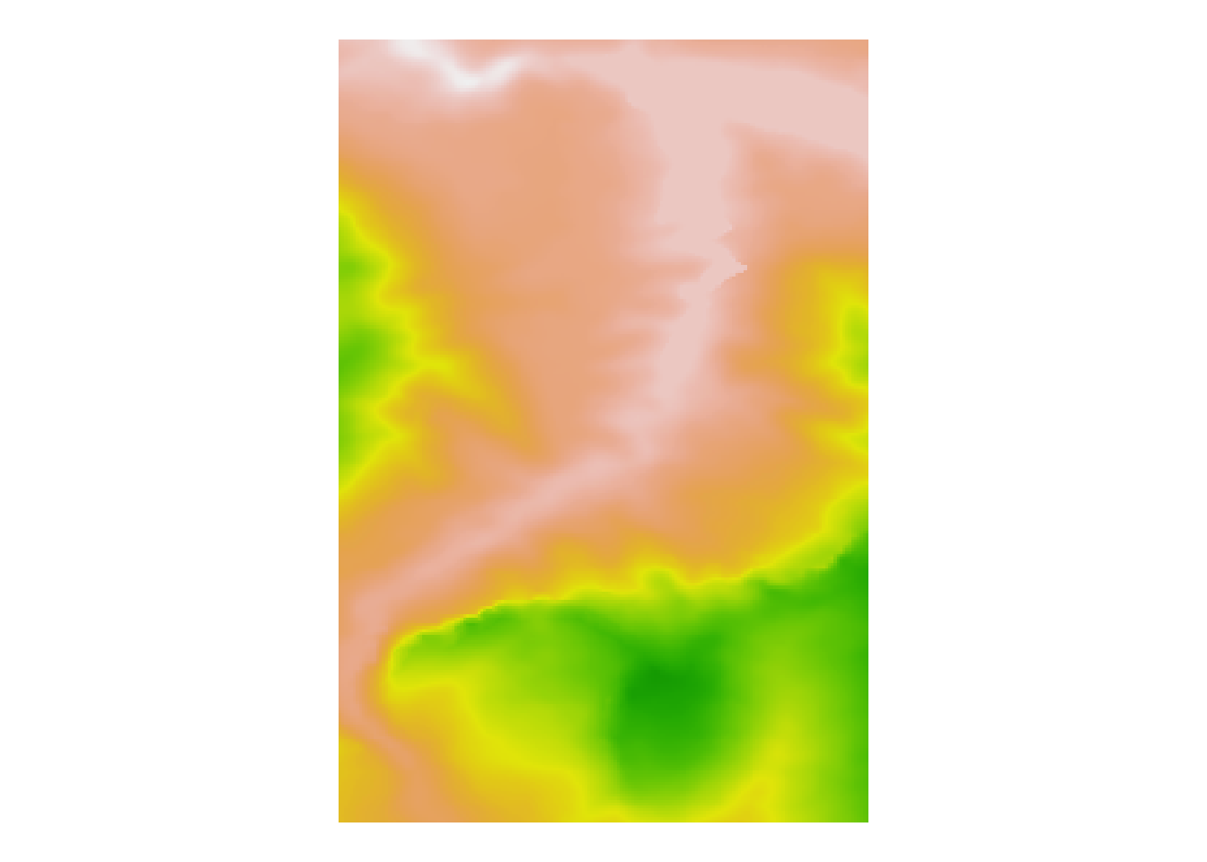
7.2.4 Interactive Raster Previews with plainview
The plainview R package provides an interactive HTML viewer, much as we might use to present an interactive map, for previewing raster images. The viewer supports zooming and panning and can also detect mouse location information.
The plainview::plainView() function provides a straightforward way of rendering a raster object in the interactive viewer:
library(plainview)

plainView(elev_img, legend = FALSE, verbose=FALSE)
The output seems to not work properly with bookdown. A navigation bar appears at the top of the bookdown content frame.
If a raster image is very large, this can provide a convenient way of reviewing it.
We can also overlay a raster image as a semi-transparent overlay on a map using the mapview::mapview() function:
library(mapview)
mapview(elev_img)
7.2.5 Saving the Image Raster Data to a Local File
In cases where we download the image raster into memory, rather than as an image file, we can save it out to a raster file and then load it in as a local file on future occasions, rather than having to retrieve it again from its online source.
We can save the raster image as a tif file:
stage_tif = "stage_elevation.tif"

# elev_img is a DEM, digital elevation model
# It may be more convenient to reference it as such
dem = elev_img

# Write the data to an elevation data raster tif
raster::writeRaster(elev_img, stage_tif, overwrite= TRUE)

# Load the raster image back in
elev_tif <- raster::raster(stage_tif)

# Get the dimensions in pixels?
dim <- dim(elev_tif)

elev_matrix <- matrix(
      raster::extract(elev_img, raster::extent(elev_img), buffer = 1000),
      nrow = ncol(elev_img), ncol = nrow(elev_img)
)

# Preview the raster image
plot(elev_tif)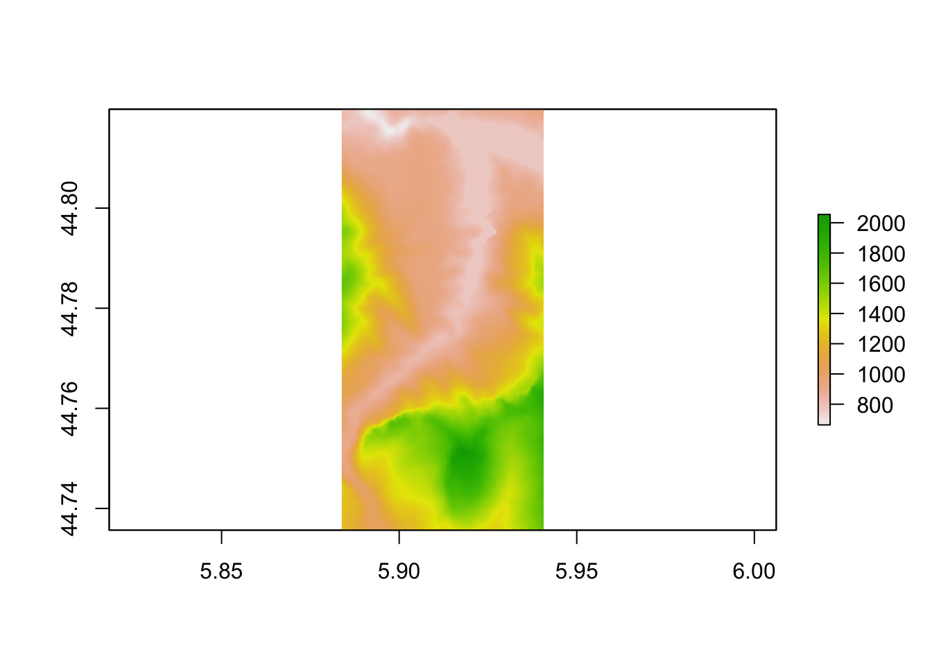
7.2.6 From raster to terra
The raster package has a long history and as such is widely encountered in examples of how to work with raster images. However, the more recent terr R package (docs), maintained via the rspatial Github organisation, looks like it may be set to challenge the raster package due its presumably closer integration with other rspatial maintained packages.
library(terra)

r <- terra::rast(stage_tif)

plot(r, main='Elevation raster via terra')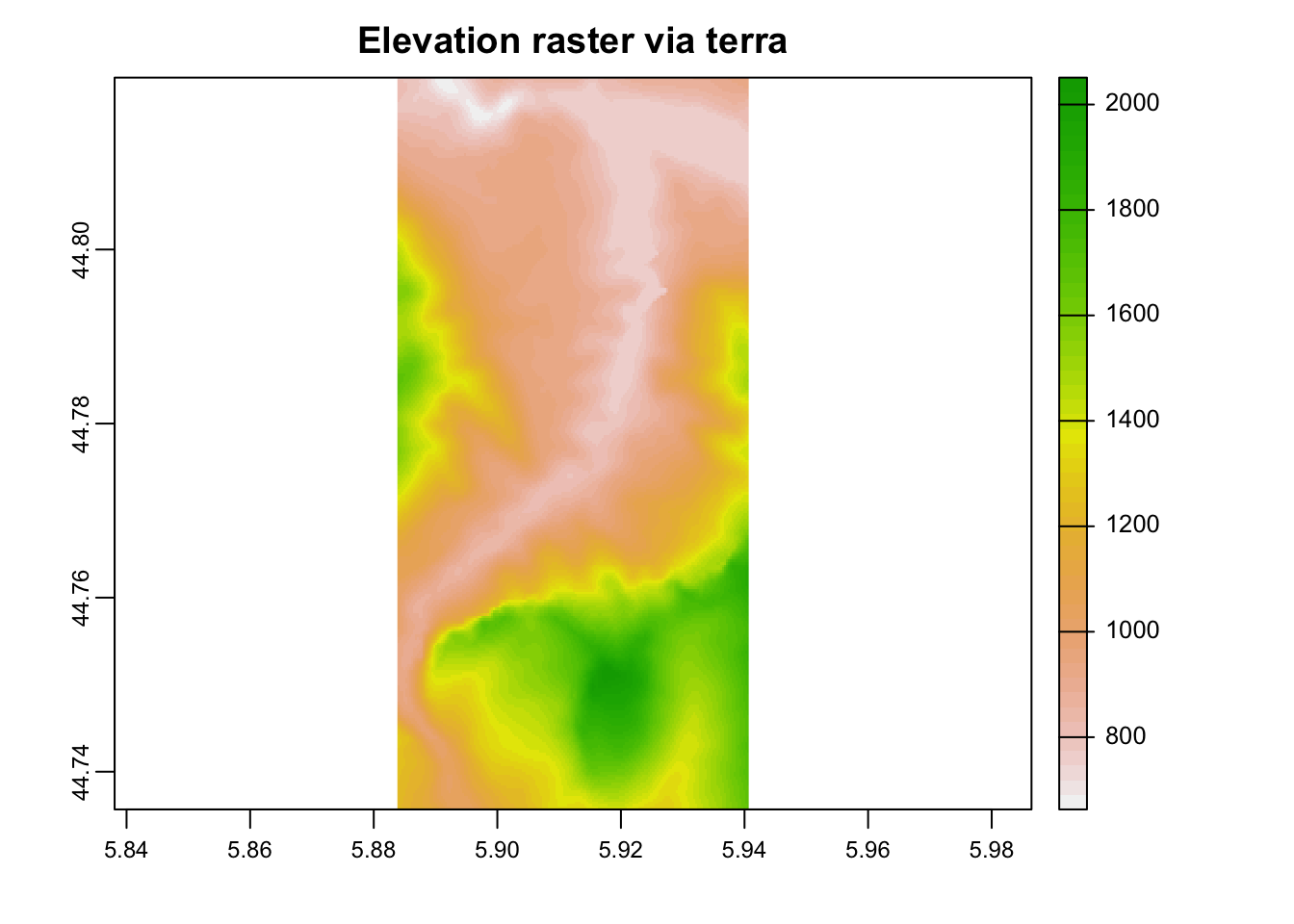
7.3 Overlaying Raster Images on Leaflet Maps
One way of checking that the raster covers the area of interest is to preview this image as a raster overlay on a leaflet map:
library(leaflet)
# Although we import the leaflet package, let's also prefix
# the functions imported from that package explicitly

pal <- leaflet::colorNumeric(c("#0C2C84", "#41B6C4", "#FFFFCC"), # span of values in palette
                    values(elev_img), #range of values
  na.color = "transparent")

leaflet() %>%
  addProviderTiles("OpenTopoMap", group = "OSM") %>%
  addRasterImage(elev_img,
                 color=pal,
                 opacity = 0.6) %>%
  leaflet::addLegend(values = values(elev_img),
                     pal = pal,
                     title = "Digital elevation model") %>%
  leaflet::addPolylines(color = "red",
                        weight = 5,
                        data=geojson_sf[1,])
7.4 Retrieving Descriptive Information About the Raster
We can retrieve the extent of the raster image using the raster::extent() function:
dem_extent = extent(dem)
dem_extent
## class : Extent
## xmin : 5.883827
## xmax : 5.94068
## ymin : 44.73566
## ymax : 44.81975Individual values can be retrieved from the extent class object using the base::attr() function:
attr(dem_extent, 'xmin')## [1] 5.883827In general, the coordinate system used to represent the x and y co-ordinates uses the same units for the x and y dimension. However, a different measurement unit may be used describe the elevation. The zscale parameter can be used to scale the elevation (z) units relative to the base x/y units. When creating a 3D plot, setting the zscale value allows us to render a “true” representation of the landscape, where the elevation (z co-ordinate) is in proportion to the x/y co-ordinates. Decreasing the zscale value increases the “spikiness” of the elevation, and allows us emphasise relief where the elevation changes are slight. Increasing the zscale value squashes the relief and flattens the rendered view.
The geoviz::raster_zscale() function returns the “true” z-scale value for a raster that keeps the x, y and z scale co-ordinates in proportion in a 3D rendered view:
# Get the zscale from the DEM

auto_zscale = geoviz::raster_zscale(elev_img)
auto_zscale
## [1] 11.80221We can use the raster::crs() or raster::projection() functions to return the co-ordinate system used by a raster, optionally returning the object as a text string:
raster::crs(dem, asText = TRUE)## [1] "+proj=longlat +datum=WGS84 +no_defs"7.4.1 Using Mapzen to Retrieve DEM raster data
We can source DEM raster data without the need for an API key from Amazon Public Datasets using MapZen.
The geoviz::mapzen(lat, long, square_km*, width_buffer*) function retrieves rasters based on a bottom left corner lat-long and a specified extent. The lat and long parameters take either a single WGS84 point to use as the centre for a square_km sized raster, or a vector of track points. Where a single location is provided, the square_km parameter takes the side length of the square to be covered by the raster. Where multiple points are provided, the width_buffer defines buffer distance in km around the points.
For example, we can retrieve a square raster covering the stage area by defining a square extent around a central location on the stage (the centroid of the stage data):
# Set an explicit side length in km
square_km = 6

stage_centroid = sf::st_centroid(geojson_sf[1,]) %>%
                      sf::st_geometry() %>%
                      sf::st_coordinates()

#Make sure we pass the co-ordinates in in the correct order
dem <- geoviz::mapzen_dem(stage_centroid[1,2],
                          stage_centroid[1,1],
                          square_km=square_km)

raster::plot(dem)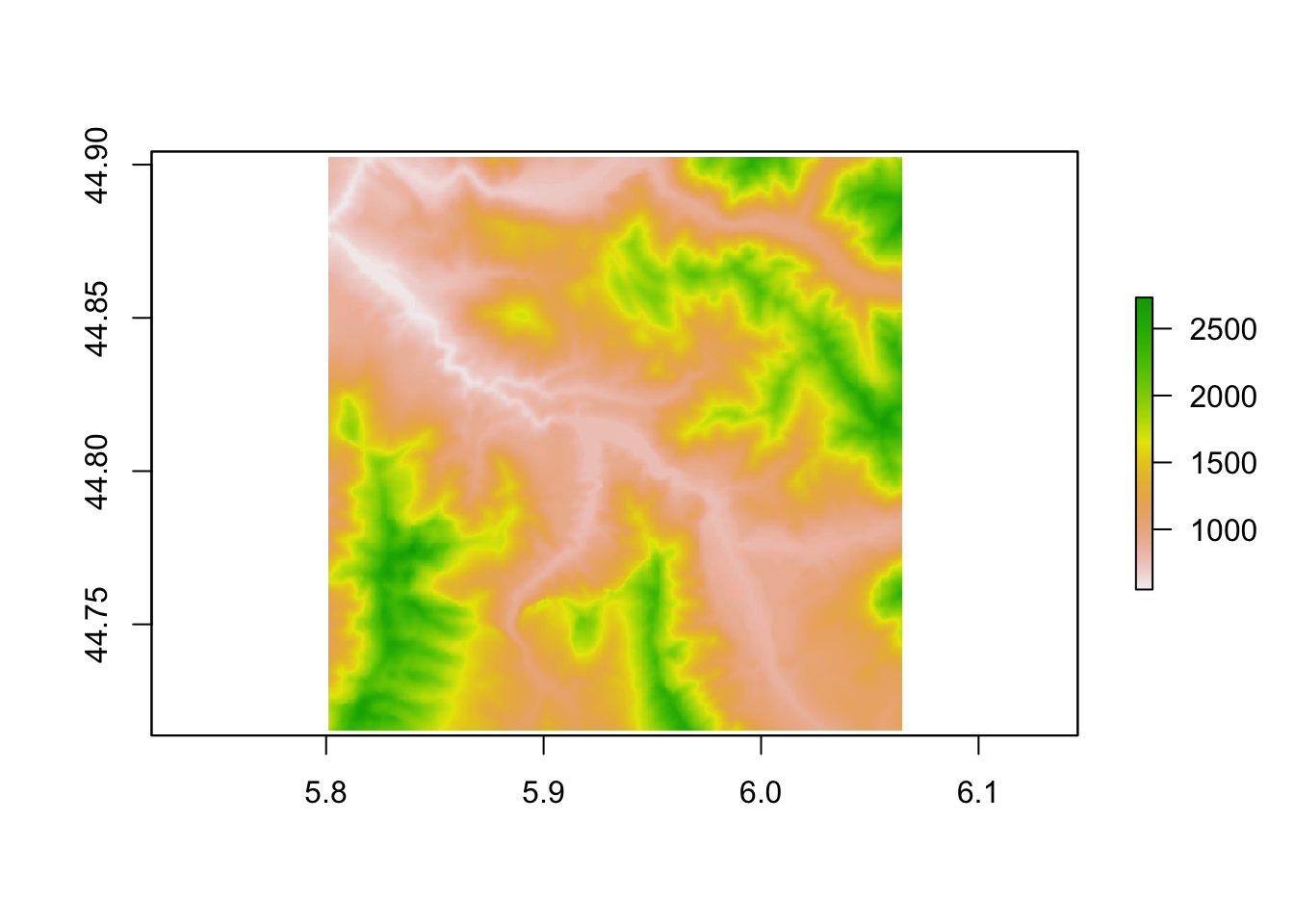
7.4.1.1 Retrieving Stage Level Mapzen Elevation Data
To retrieve data for a particular stage, we might alternatively identify all the co-ordinates in a stage and then retrieve an elevation raster that at least covers the extent of all points buffered by a particular amount:
# Get stage co-ordinates
stage_coords = as.data.frame(sf::st_coordinates(geojson_sf[1,]))

# Retrieve elevation raster buffered to 0.5km extent
dem2 <- geoviz::mapzen_dem(stage_coords$Y, stage_coords$X,
                           width_buffer=0.5)

raster::plot(dem2)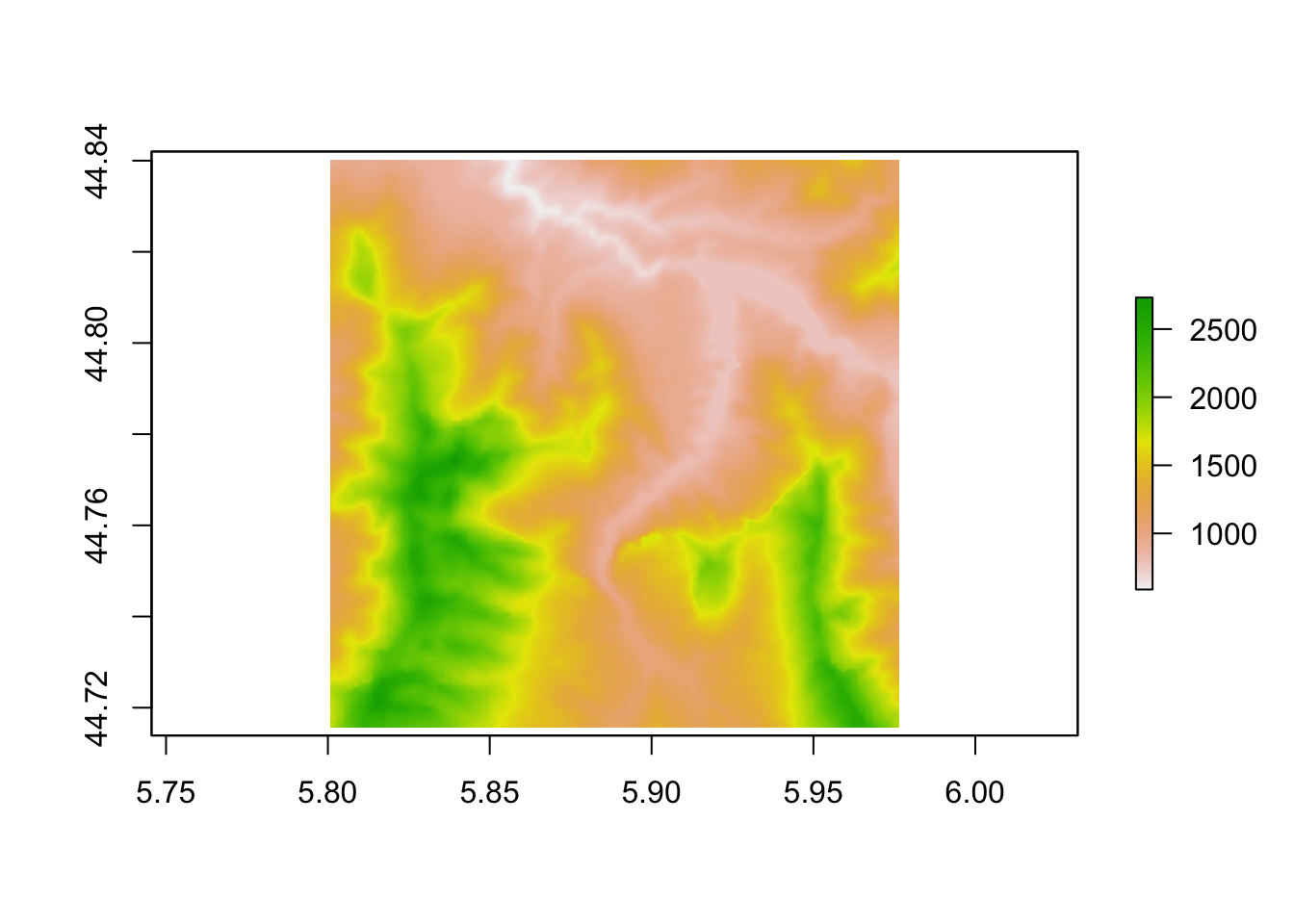
We can check we have got the co-ordinates in the correct order, and are using an appropriate buffer distance, by overplotting the raster on a leaflet map and making sure it covers the area of interest:
pal <- colorNumeric(c("#0C2C84", "#41B6C4", "#FFFFCC"),
                    values(elev_img), #range of values
                    na.color = "transparent")

leaflet() %>%
  addProviderTiles("OpenTopoMap", group = "OSM") %>%
  addRasterImage(dem,
                 color=pal,
                 opacity = 0.6) %>%
  addLegend(values = values(dem),
            pal = pal,
            title = "Digital elevation model") %>%
  addPolylines(color = "red", weight = 5,
               data=geojson_sf[1,])
7.4.1.2 Setting a Square Side Value
If we want to retrieve the data using a square side value, we can derive it from the stage bounding box by setting the square side to the longer of the width or the height of the bounding box.
Since the square side needs to be in meters, we need to either retrieve the bounding box from a projection where the units are meters, or, for the likes of the WGS84 / latlong projection where the units are in degrees, use a function that can determine the distance in meters rather than degrees.
In the first case, if we know the UTM zone for our location of interest, we can transform the stage co-ordinates to the UTM projection and get the bounding box in meters:
utm_proj_string = "+proj=utm +zone=32 +datum=WGS84 +units=m +no_defs"

stage_bbox = sf::st_bbox(sf::st_transform(geojson_sf[1,],
                                          crs=utm_proj_string))

stage_bbox
## xmin ymin xmax ymax
## 253330.9 4958273.8 258123.2 4967513.3We can then calculate the square side as the longer of the bounding box sides:
stage_bbox[['xmax']] - stage_bbox[['xmin']]## [1] 4792.326stage_bbox[['ymax']] - stage_bbox[['ymin']]## [1] 9239.405In the second case, we have the bounding box in degrees:
sf::st_bbox(geojson_sf[1,])## xmin ymin xmax ymax
## 5.883753 44.735616 5.940715 44.819732To simplify things, let’s create a function to get the corners:
get_corners = function(stage_bbox) {

  bottom_left = cbind(stage_bbox[['xmin']], stage_bbox[['ymin']])
  top_left = cbind(stage_bbox[['xmin']], stage_bbox[['ymax']] )
  bottom_right = cbind(stage_bbox[['xmax']], stage_bbox[['ymin']] )

  rbind(bottom_left, top_left, bottom_right)
}
Return the corners:
corners = get_corners(sf::st_bbox(geojson_sf[1,]))

bottom_left = corners[1,]
top_left = corners[2,]
bottom_right = corners[3,]
To calculate the distance in meters, rather than degrees, we can use a quick Haversine distance function such as geosphere::distHaversine() to look up the distance as a great circle distance on a spherical representation of the Earth. This is likely to be “good enough” for short distances:
geosphere::distHaversine(bottom_left, top_left) # vertical side## [1] 9363.75geosphere::distHaversine(bottom_left, bottom_right) # horizontal side## [1] 4504.392Alternatively, we can use the more accurate, but more computationally intensive, geosphere::distVincentyEllipsoid() Vincenty distance calculation on an ellipsoid representation of the Earth:
a = 6378137 # Equatorial axis of ellipsoid
b = 6356752.3142 # Polar axis of ellipsoid
f = 1/298.257223563 # Inverse flattening of ellipsoid

geosphere::distVincentyEllipsoid(bottom_left, top_left,
                                 a=a, b=b, f=f)
## [1] 9347.595geosphere::distVincentyEllipsoid(bottom_left, bottom_right,
a=a, b=b, f=f)## [1] 4511.88Distances in meters can also be returned by calling thesp::spDists() or sp::spDistsN1() function:
# Calculate the length of each side as the distance between two points
# The spDistsN1() function takes a matrix of points and a comparison point
# and then returns the distance from each point in the matrix
# to the comparison point
# great circle on WGS84 ellipsoid)

sp::spDistsN1(matrix(rbind(bottom_right, top_left), nrow=2),
              bottom_left, longlat=TRUE)
## [1] 4.511874 9.347687One thing we notice from all these techniques is that they give slightly different values for the distance measures. Whilst this doesn’t create too many problems for the current use cases, if we demand accuracy then it may be problematic. Either I’m doing something wrong, or you need to be really sure what calculation method is being applied and what parameter values (eg for the Earth ellipsoid) are being used.
7.4.2 Additional Elevation Data Downloading Tools
Additional tools for download elevation data can be found here:
- Interline PlanetUtils: Dockerised tools for downloading and merging GeoTIFF elevation rasters.
7.5 Manipulating Raster Images
One of the more useful techniques for working with raster images is the ability to add a buffer area around the raster by padding the raster margins.
One way of adding a buffer is to redefine the raster extent using the raster::extent() function:
e0=extent(elev_img)
# Top/bottom and left/right side
#raster::plot(extend(elev_img, c(100,20), value = 0))
e2 = extent(attr(e0,'xmin')-0.1, attr(e0,'xmax')+0.05,
            attr(e0,'ymin'), attr(e0,'ymax')+0.1)
#attr(extent(elev_img),'xmin') = attr(extent(elev_img),'xmin') -0.5
raster::plot(extend(elev_img, e2, value = 0))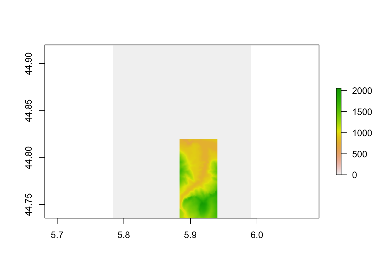
Changing the extent requires us to know the original extent and then extend is using the appropriate coordinate system.
A simpler approach is to use the following modify_raster_margins() function retrieved from the spatial.tools package that appears to have been removed from CRAN. This function lets you add a specified number of rows or columns of padding, as appropriate, to each dimension:
# From spatial.tools - no longer on CRAN?
#' Add/subtract rows and columns from Raster*
#'
#'
#' @param x A Raster* object.
#' @param extent_delta Numeric vector. How many rows/columns to add/subtract to the left,right,top, and bottom of an image.  Default is c(0,0,0,0) (no change).
#' @param value Value to fill in when adding rows/columns.
#' @return A Raster* object.
#' @author Jonathan A. Greenberg
#' @details A quick way to add/subtract margins from a Raster* object.  extent_delta is a four-element integer vector that
#' describes how many rows/columns to add to the (left,right,top,bottom) of the image (in that order).  Negative values remove rows,
#' positive values add rows.
#'
#' @examples
#' tahoe_highrez <- brick(system.file("external/tahoe_highrez.tif", package="spatial.tools"))
#' dim(tahoe_highrez)
#' # Remove one row and column from the top, bottom, left, and right:
#' tahoe_highrez_cropped <- modify_raster_margins(x=tahoe_highrez,extent_delta=c(-1,-1,-1,-1))
#' dim(tahoe_highrez_cropped)
#' # Add two rows to the top and left of the raster, and fill with the value 100.
#' tahoe_highrez_expand <- modify_raster_margins(x=tahoe_highrez,extent_delta=c(2,0,2,0),value=100)
#' dim(tahoe_highrez_expand)
#' @import raster
#' @export

modify_raster_margins <- function(x,extent_delta=c(0,0,0,0),value=NA)
{
    x_extents <- extent(x)
    res_x <- res(x)

    x_modified <- x

    if(any(extent_delta < 0))
    {
        # Need to crop
        # ul:
        ul_mod <- extent_delta[c(1,3)] * res_x
        ul_mod[ul_mod > 0] <- 0
        lr_mod <- extent_delta[c(2,4)] * res_x
        lr_mod[lr_mod > 0] <- 0
    # This works fine, but for some reason CRAN doesn't like it:
    #   crop_extent <- as.vector(x_extents)
        crop_extent <- c(x_extents@xmin,x_extents@xmax,x_extents@ymin,x_extents@ymax)
        crop_extent[c(1,3)] <- crop_extent[c(1,3)] - ul_mod
        crop_extent[c(2,4)] <- crop_extent[c(2,4)] + lr_mod

        x_modified <- crop(x_modified,crop_extent)
    }

    if(any(extent_delta > 0))
    {
        # Need to crop
        # ul:
        ul_mod <- extent_delta[c(1,3)] * res_x
        ul_mod[ul_mod < 0] <- 0
        lr_mod <- extent_delta[c(2,4)] * res_x
        lr_mod[lr_mod < 0] <- 0
#       Again, a hack for CRAN?
#       extend_extent <- as.vector(x_extents)
        extend_extent <- c(x_extents@xmin,x_extents@xmax,x_extents@ymin,x_extents@ymax)
        extend_extent[c(1,3)] <- extend_extent[c(1,3)] - ul_mod
        extend_extent[c(2,4)] <- extend_extent[c(2,4)] + lr_mod

        x_modified <- extend(x_modified,extend_extent,value=value)
    }

    return(x_modified)
}
We can then add margins around a raster image with a specified pixel extent:
elev_img_margin = modify_raster_margins(elev_img, c(100,100,25,200), 5000)
plot(elev_img_margin)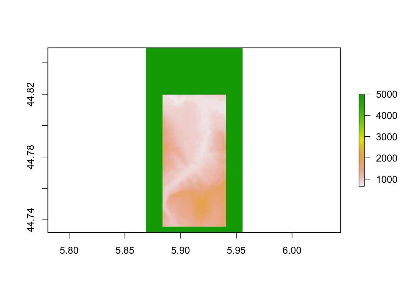
7.6 Ridge maps
If you’re an aficionado of fantasy novels, you’re probably familiar with ridge maps, woodcut style views of mountainous landscapes that provide the setting for many a heroic tale or adventure.
library(ggplot2)

# eg via https://udurrani.netlify.app/posts/2020-12-25-elevation-maps-in-r/
library(ggridges)

need_raster_df = data.frame(sampleRegular(elev_img, 10000, xy=TRUE))
names(need_raster_df) = c('x', 'y', 'elevation')
ggr = ggplot()

ggr = ggr +
      geom_density_ridges(data = need_raster_df,
                          aes(x, y,
                              group=y,
                              height = elevation),
                          stat = "identity", scale=100,
                          fill="black", color="white") +
      theme_void() +
      theme(panel.background = element_rect(fill = "black"),
            plot.background = element_rect(fill = "black"))

ggr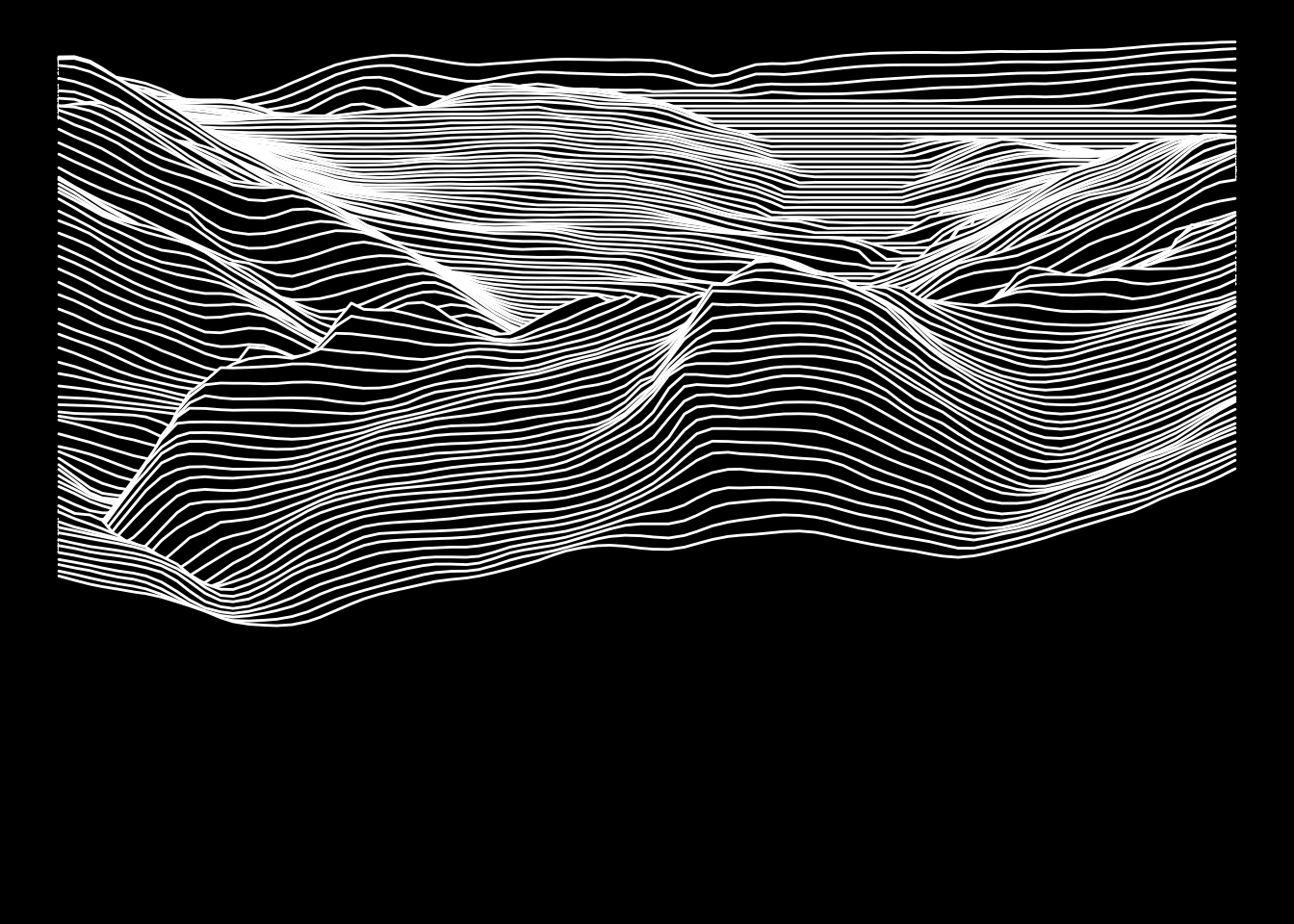
By default we are taking lines across the raster matrix, essentially giving us a view from the south. If we rotate matrix 90 degrees by finding its transpose, we can essentially view the scene from the west.
7.7 Further Information
We will explore various ways of working with elevation raster images in more detail in a later chapter.
It is also worth noting that additional tools for working with raster images may be provided in other R packages. For example, the rasterVis package provides additional tools for visualising data over 2D rasters although the tools used in that package are not of immediate relevance here.