10 Overlaying 2D rayshader Maps
In this chapter, we will explore in more detail how we can add overlays to rayshader two-dimensional maps such as water feature overlays, map tiles or stage routes.
10.1 Load in Base Data
As ever, let’s load in our stage data:
geojson_filename = 'montecarlo_2021.geojson'
geojson_sf = sf::st_read(geojson_filename)
## Reading layer `montecarlo_2021' from data source `/Users/tonyhirst/Documents/GitHub/visualising-rally-stages/montecarlo_2021.geojson' using driver `GeoJSON'
## Simple feature collection with 9 features and 2 fields
## geometry type: LINESTRING
## dimension: XY
## bbox: xmin: 5.243488 ymin: 43.87633 xmax: 6.951953 ymax: 44.81973
## geographic CRS: WGS 84And also load in the elevation data raster:
library(raster)
library(rayshader)

# Previously downloaded TIF digital elevation model (DEM) file
stage_tif = "stage_elevation.tif"

# Load in the previously saved image raster
elev_img = raster(stage_tif)

# Note we can pass in a file name or a raster object
elmat = raster_to_matrix(stage_tif)
10.2 Adding overlays
The rayshader package includes various tools for styling the rendering of the 2d image.
10.2.1 Adding Shadows to rayshader Maps
It can often be convenient to construct shadow layers for a particular rayshader map that we can add to the rendering as required:
# Add shade
raymat <- ray_shade(elmat, zscale = auto_zscale, lambert = TRUE)
# And "ambient occlusion shadow"
ambmat <- ambient_shade(elmat, zscale = auto_zscale)
The shading functions accept sunaltitude and sunangle paramters to specify the sun / light source position. The suncalc R package can be used to determine sun altitude and and angle settings for a particular date and time at a specified location.
We can also create a composite shadow layer constructed from several shadow operators piped together:
# More shadow style from:
# https://www.tylermw.com/adding-open-street-map-data-to-rayshader-maps-in-r/

# We can build up layers that can be generated once then added
# as overlays to construct views from basic parts
shadow_layer = height_shade(elmat) %>%
  add_overlay(sphere_shade(elmat, texture = "desert",
                           zscale=auto_zscale, colorintensity = 5), alphalayer=0.5) %>%
  add_shadow(lamb_shade(elmat, zscale = auto_zscale),0) %>%
  add_shadow(texture_shade(elmat,detail=8/10,contrast=9,brightness = 11), 0.1)
The layers can be added to the rayshader map in the normal way:
# Add water
watermap <- detect_water(elmat, zscale = 8)

demo_map = elmat %>%
              add_overlay(shadow_layer)  %>%
              add_water(watermap, color = "desert")

demo_map %>%
  plot_map()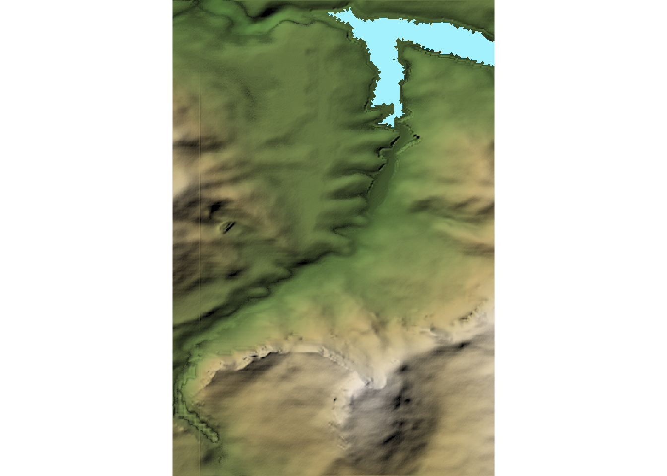
10.2.1.1 Retrieving Shadow Data Along a Route
If we can access just the shadow layer data, one interesting possibility is that we could produced a “shadow depth” profile of a route identifying which bit are in shadow at a particular time and date.
10.2.2 Adding Water Features
We can detect water (and even modify the height of the water to model raising water levels) to create a layer that we can later add to the rendered map.
# Add water
watermap <- detect_water(elmat, zscale = 8)
Let’s add that layer to the 2d map:
# Texture palettes:
# `imhof1`,`imhof2`,`imhof3`,`imhof4`,`bw`,`desert`, and `unicorn`
elmat %>%
  #sphere_shade(texture = "imhof1") %>%
  # Optionally set sun angle
  sphere_shade(sunangle = -45, texture = "imhof1") %>%
  add_water(watermap, color = "bw") %>%
  plot_map()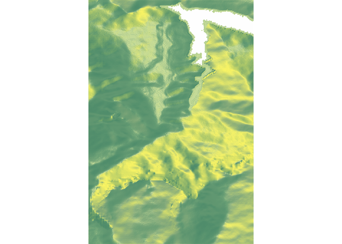
10.2.3 Overlaying Map Tiles
We can also add tiles as an overlay.
For example, the geoviz package provides a way for us to retrieve popular map tilesets and then overlay them onto the rayshader map.
Let’s grab some tiles covering the extent of our original raster image and create overlays from them:
# via https://github.com/neilcharles/geoviz
library(geoviz)

# stamen: toner, watercolor, terrain
overlay_image_watercolor <-
  slippy_overlay(elev_img,
                 image_source = "stamen",
                 image_type = "watercolor",
                 png_opacity = 0.5)

overlay_image_tonerlite <-
  slippy_overlay(elev_img,
                 image_source = "stamen",
                 image_type = "toner",
                 png_opacity = 0.5)

overlay_image_terrain <-
  slippy_overlay(elev_img,
                 image_source = "stamen",
                 image_type = "terrain",
                 png_opacity = 0.9)
We can now overlay a tileset onto the rendered map.
In the following example, notice how I have further separated out the map creation phase from the map plotting phase:
scene <- elmat %>%
  sphere_shade(sunangle = 270, texture = "desert") %>%
  add_overlay(overlay_image_watercolor)

scene  %>%
  plot_map()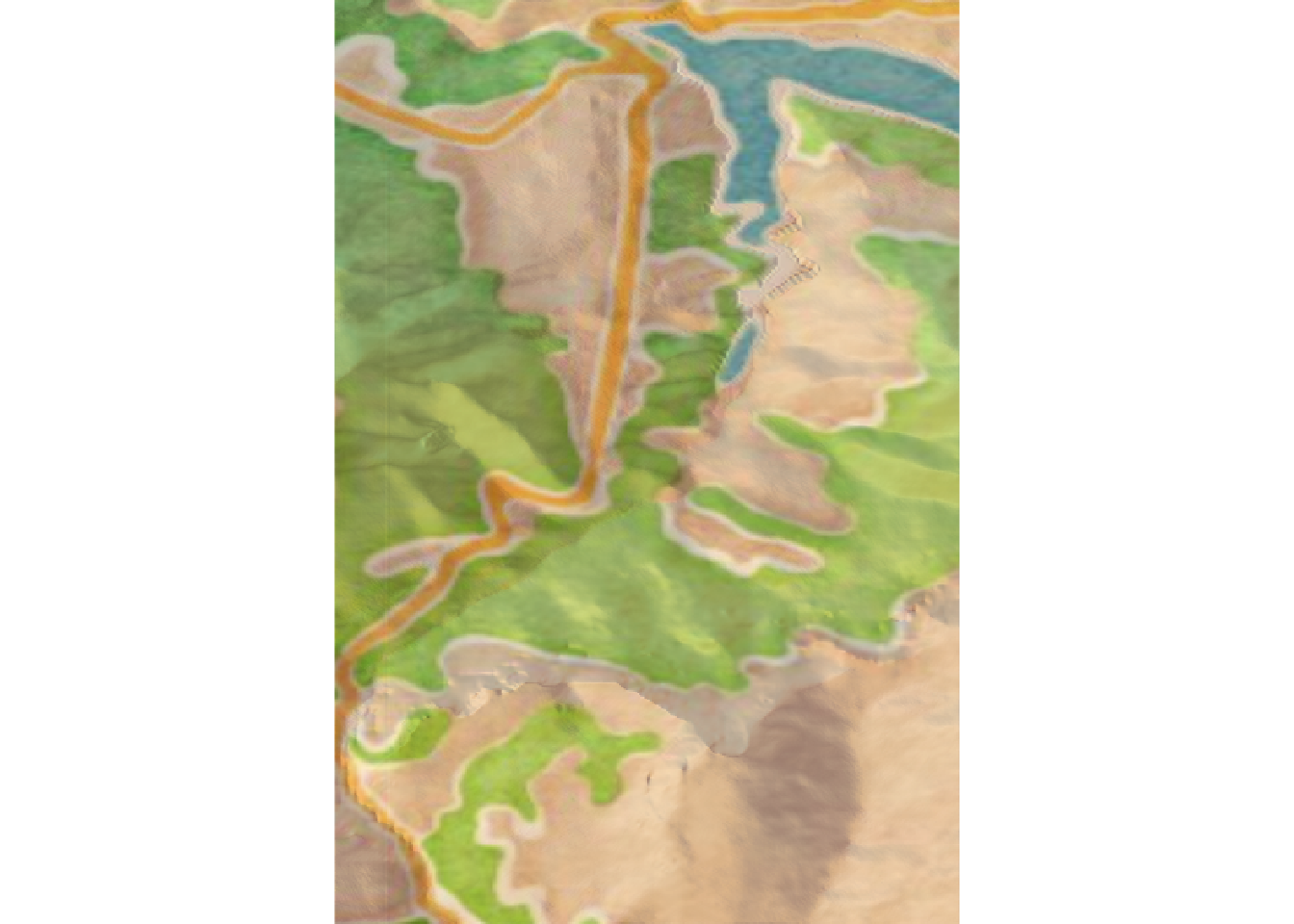
10.2.3.1 Setting Elevation Sensitive Tile Transparancy
We can also specify different elevations at which we want to apply an overlay as a transparency.
For example, we can turn mountainous parts of the overlay transparent, showing the tiles overlaid on the lower altitude areas but not on the higher regions, which in this case are rendered with a black and white texture:
overlay_image_tonerlite_low_alt <-
  elevation_transparency(overlay_image_terrain,
                        elev_img,
                        pct_alt_high = 0.5,
                        alpha_max = 0.9)

scene <- elmat %>%
  sphere_shade(sunangle = 270, texture = "bw") %>%
  add_overlay(overlay_image_tonerlite_low_alt) %>%
  plot_map()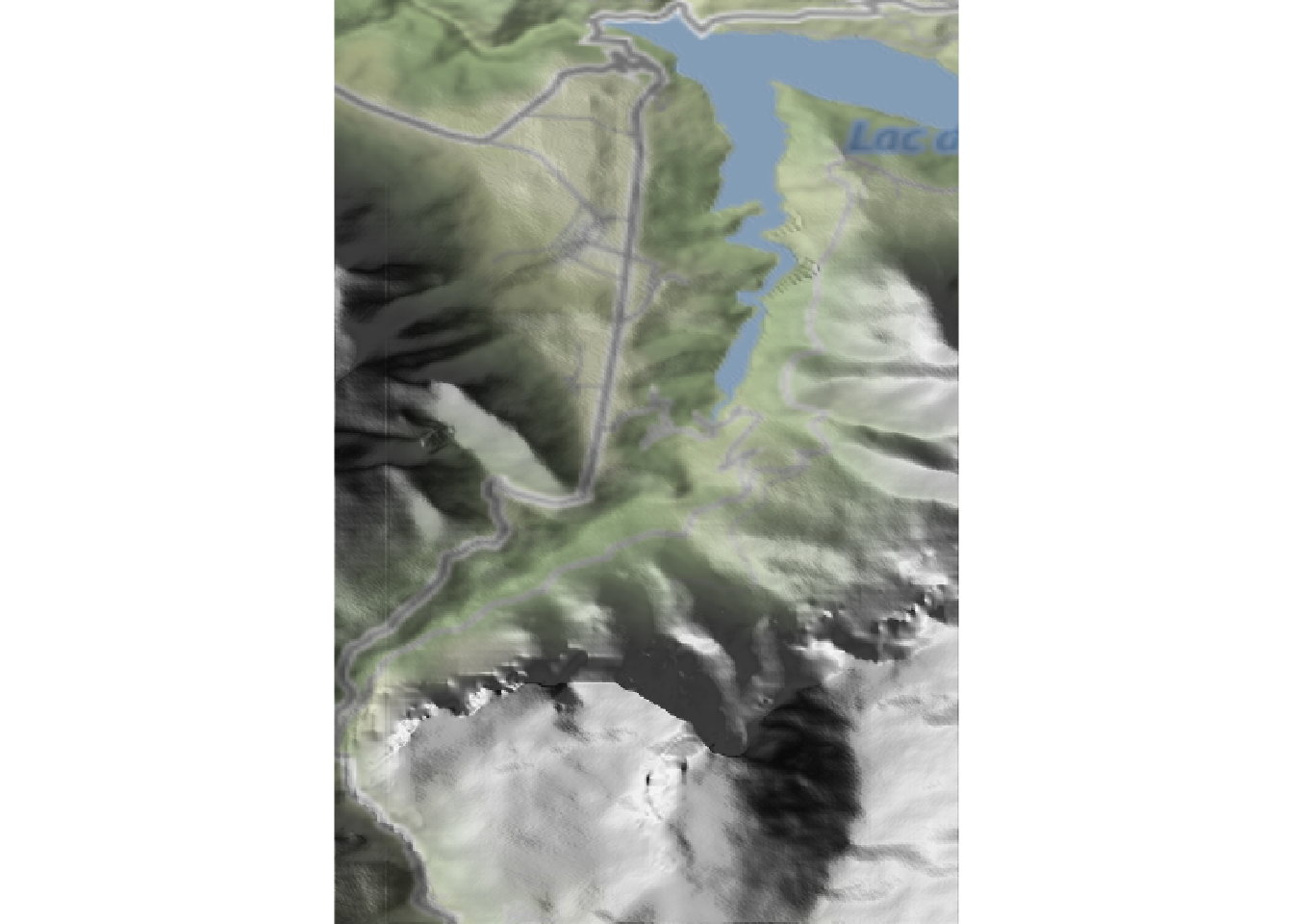
10.3 Adding a Stage Route Layer
When adding overlays, we ofter need to specify the extent of the area covered by the overlay.
For our stage route, we can take the extent directly from the geojson loaded data:
library(sf)

extent(st_bbox(geojson_sf[1,]))
## class : Extent
## xmin : 5.883753
## xmax : 5.940715
## ymin : 44.73562
## ymax : 44.81973We can then create a route layer as a line overlay:
yellow_route = generate_line_overlay(geojson_sf[1,],
                                    extent = extent(geojson_sf[1,]),
                                    heightmap = elmat,
                                    linewidth = 5, color="yellow")
We can add the line overlay to our map to show the path followed by the stage route:
mapped_route_yellow = elmat %>%
  sphere_shade(sunangle = -45, texture = "bw") %>%
  #add_water(watermap, color = "bw") %>%
  add_overlay(yellow_route)

mapped_route_yellow %>%
  plot_map()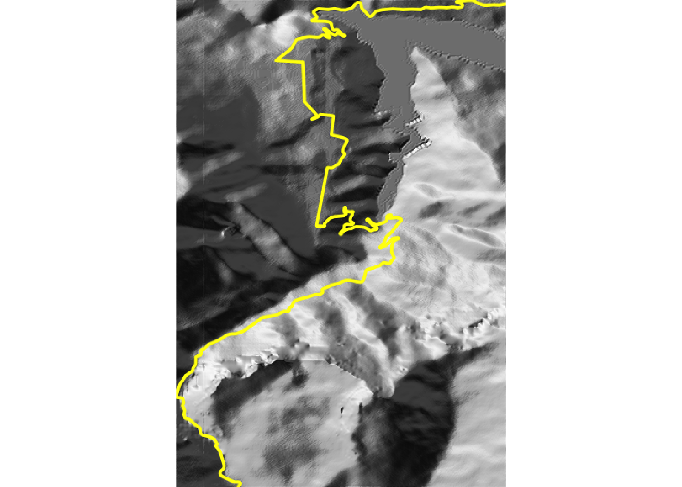
The geoviz::add_gps_to_rayshader() can also add a route to a rayshader model from longitude, latitude and elevation vectors.
10.3.1 Buffering the Stage Route View
One problem with that view is that the route extent borders on the edge of the rendered image. It would be easier to see the route if the extent of the image was increased to provide a bordered area around the route.
We can create a “buffered boundary box” around the stage extent as follows:
library(spatialEco)

bb_sp = SpatialPoints(extent(geojson_sf[1,]))
proj4string(bb_sp) <- st_crs(geojson_sf[1,])$proj4string

# Create a new, buffered region
stage_bbox_buffered = st_bbox(geo.buffer(x=bb_sp, r=500))
stage_bbox_buffered
## xmin ymin xmax ymax
## 5.877431 44.731117 5.947037 44.824231We can then use those extended bounds to retrieve a buffered elevation raster image:
ex.df2 <- data.frame(x= c(stage_bbox_buffered[['xmin']],
                          stage_bbox_buffered[['xmax']]),
                    y= c(stage_bbox_buffered[['ymin']],
                         stage_bbox_buffered[['ymax']]))

library(elevatr)

# The zoom level, z, impacts on how long it takes to download the imagery
# z ranges from 1 to 14
# https://www.rdocumentation.org/packages/elevatr/versions/0.3.4/topics/get_elev_raster
prj_dd <- "+proj=longlat +ellps=WGS84 +datum=WGS84 +no_defs"
elev_img2 <- get_elev_raster(ex.df2, prj = prj_dd, z = 12, clip = "bbox")
## Mosaicing & Projecting## Clipping DEM to bbox## Note: Elevation units are in meters.
## Note: The coordinate reference system is:
## GEOGCRS["unknown",
## DATUM["World Geodetic System 1984",
## ELLIPSOID["WGS 84",6378137,298.257223563,
## LENGTHUNIT["metre",1]],
## ID["EPSG",6326]],
## PRIMEM["Greenwich",0,
## ANGLEUNIT["degree",0.0174532925199433],
## ID["EPSG",8901]],
## CS[ellipsoidal,2],
## AXIS["longitude",east,
## ORDER[1],
## ANGLEUNIT["degree",0.0174532925199433,
## ID["EPSG",9122]]],
## AXIS["latitude",north,
## ORDER[2],
## ANGLEUNIT["degree",0.0174532925199433,
## ID["EPSG",9122]]]]# Save out the buffered image
stage_tif = "buffered_stage_elevation.tif"
# Write the data to an elevation data raster tif
raster::writeRaster(elev_img2, stage_tif, overwrite= TRUE)
elmat_buffered = raster_to_matrix(elev_img2)To create a buffered yellow route, we generate the line overlay with an extend matching that of the buffered image and the heightmap associated with that image:
yellow_route_b = generate_line_overlay(geojson_sf[1,],
                                       extent = extent(elev_img2),
                                       heightmap = elmat_buffered,
                                       linewidth = 5, color="yellow")
Plotting the buffered route in the buffered image now provides us with a marginal border around the edge of the route:
mapped_route_yellow = elmat_buffered %>%
  sphere_shade(sunangle = -45, texture = "bw") %>%
  add_overlay(yellow_route_b)  %>%
  plot_map()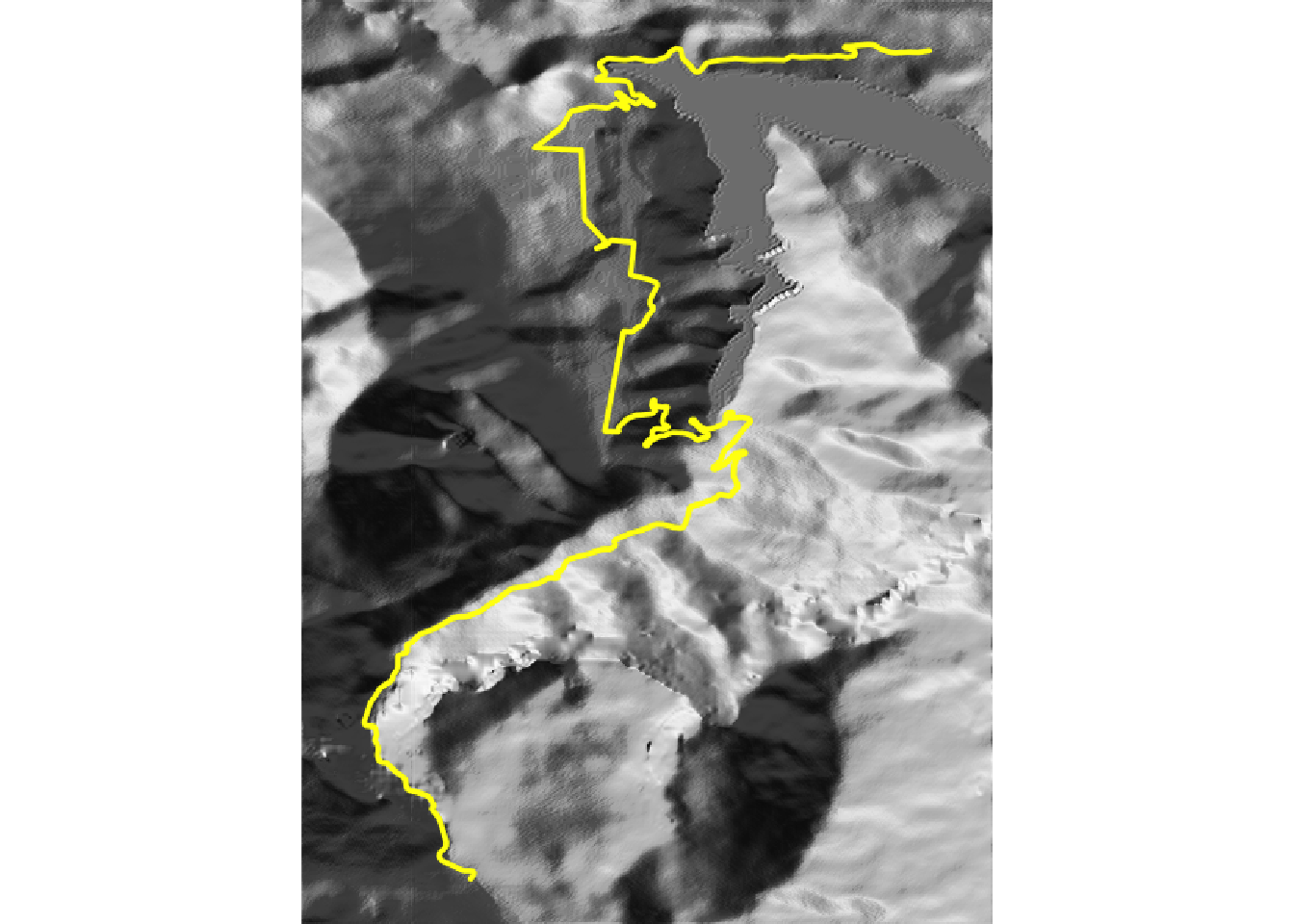
10.4 Modeling Increased Water Levels
The rayshader::plot_3d() function takes a water_depth parameter that allows us to model changing water levels. This is not really relevant to rally route analysis and visualisation, although it may be of interest in other contexts (eg raising sea levels, historical views over land that as since been reclaimed from the sea, dam bursts, etc.)