5 Introducing Map Projections

At this point, we should probably talk about coordinate reference systems (CRS) and projections…

5.1 Load in the Route Data

Let’s load in our route data to give us something to work with:

library(sf)

geojson_filename = 'montecarlo_2021.geojson'
geojson_sf = st_read(geojson_filename)

## Reading layer `montecarlo_2021' from data source `/Users/tonyhirst/Documents/GitHub/visualising-rally-stages/montecarlo_2021.geojson' using driver `GeoJSON'
## Simple feature collection with 9 features and 2 fields
## geometry type:  LINESTRING
## dimension:      XY
## bbox:           xmin: 5.243488 ymin: 43.87633 xmax: 6.951953 ymax: 44.81973
## geographic CRS: WGS 84

5.2 Previewing a Map Route

Recall how our stage map looked when we plotted the simple features geo object using ggplot() with the geom_sf() geometry:

library(ggplot2)

g_sf = ggplot(data=geojson_sf[1,]) + geom_sf() +
        theme(axis.text.x = element_text(angle = 45))
g_sf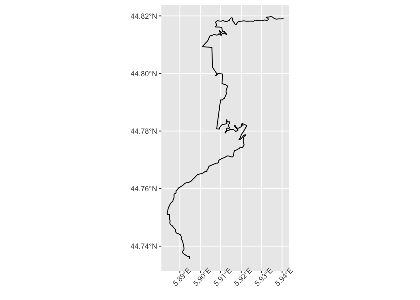

The geom_sf() geometry took into account the fact that the co-ordinates were in degrees latitude and longitude and then scaled the visual representation accordingly.

5.3 Plotting LatLong Naively

But what if we plot the coordinates just as numbers…?

We can grab the coordinates from our route using the sf::st_coordinates() function and then cast them to a dataframe:

coords_df = as.data.frame( st_coordinates(geojson_sf[1,]) )
head(coords_df)

##          X        Y L1
## 1 5.894486 44.73562  1
## 2 5.894618 44.73580  1
## 3 5.894778 44.73602  1
## 4 5.894805 44.73621  1
## 5 5.894672 44.73636  1
## 6 5.894407 44.73642  1

If we naively plot those coordinates using the [ggplot2::geom_path()] (https://ggplot2.tidyverse.org/reference/geom_path.html) geometry which ensures that we draw a line from the first point to the second, the second to the third, and so on, we get a view that is different to the original view we plotted — the route appears to be more “squashed”. Even if we ensure that the x and y scales are in unit proportion by means of the coord_fixed() constraint, the projection still look wrong:

g_ll = ggplot(coords_df, aes(x=X, y=Y)) +
          geom_path() #+ coord_fixed()

g_ll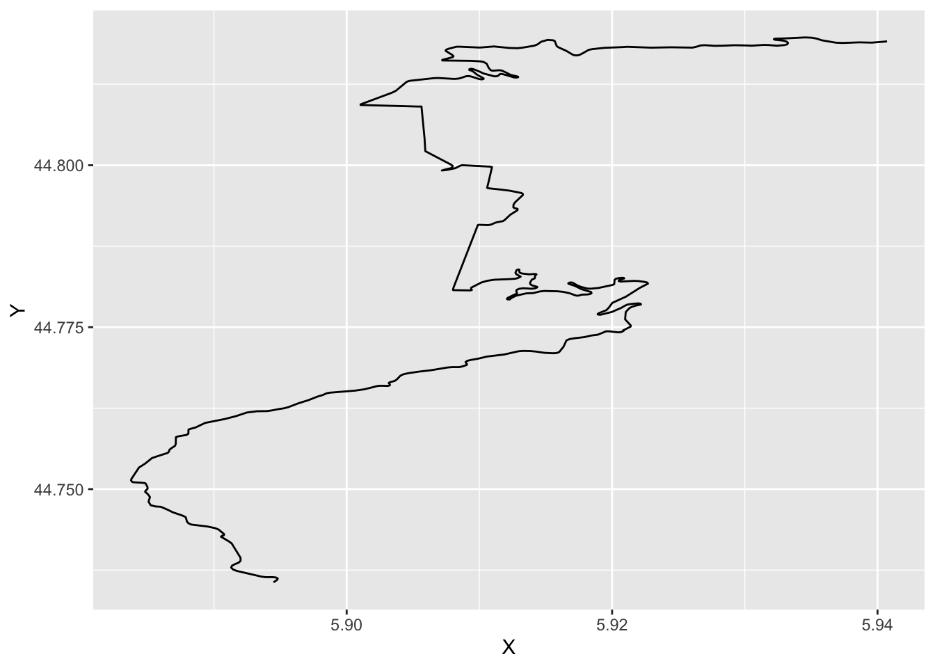

To render the “geo” view, we need to map the co-ordinates to a scale with regular units, such as meters, rather than spherical coordinates, such as degrees.

In the original object, we see that the coordinates reference system (CRS) is defined in terms of longitude and latitude:

st_crs(geojson_sf)$proj4string

## [1] "+proj=longlat +datum=WGS84 +no_defs"

5.4 Using the UTM Co-ordinate Reference System

The UTM (Universal Transverse Mercator) coordinate system uses units of meters rather than degrees. It allows us to represent spatial extents using “metric” two dimensional grid squares. To map from latlong to UTM coordinates, we need to know where on the earth a point roughly corresponds to. The world is imagined in terms of a series of zones, marked off a bit like time zones, in vertical “bands” that extend around the world.

The bands are given numerical codes according to the EPSG system that can be determined from latitude and longitude coordinates as follows:

# Detect the UTM zone as an EPSG code
lonlat2UTMzone = function(lonlat) {
  utm = (floor((lonlat[1] + 180) / 6) %% 60) + 1
  if(lonlat[2] > 0) {
    utm + 32600
  } else{
    utm + 32700
  }
}

We can define a new projection string that identities the UTM CRS and an appropriate zone using the coordinates from the starting point of our route:

# Keep track of the original proj4 string
old_crs = st_crs(geojson_sf[1,])$proj4string

# Generate a new projection in the appropriate UTM zone
crs_zone = lonlat2UTMzone(c(st_coordinates(geojson_sf[1,])[1,1],
                            st_coordinates(geojson_sf[1,])[1,2]))

new_proj4_string = st_crs(crs_zone)$proj4string
new_proj4_string

## [1] "+proj=utm +zone=31 +datum=WGS84 +units=m +no_defs"

5.4.1 Using st_transform for Projection Transformations

We can transform our route to the new projection using the sf::st_transform() function:

# Transform the route to the UTM projection
utm_routes = st_transform(geojson_sf, crs=new_proj4_string)

Now let’s look at our coordinates under this projection:

utm_df = as.data.frame(st_coordinates(utm_routes[1,]))

head(utm_df)

##          X       Y L1
## 1 729177.5 4957658  1
## 2 729187.2 4957678  1
## 3 729199.0 4957703  1
## 4 729200.4 4957724  1
## 5 729189.3 4957741  1
## 6 729168.1 4957746  1

We see the X and Y values have been transformed from their original latitude and longitude values into UTM coordinates in meters.

What happens if plot the coordinates now?

g_utm = ggplot(utm_df, aes(x=X, y=Y)) + 
          geom_path() + coord_fixed() +
          theme(axis.text.x = element_text(angle = 45))
g_utm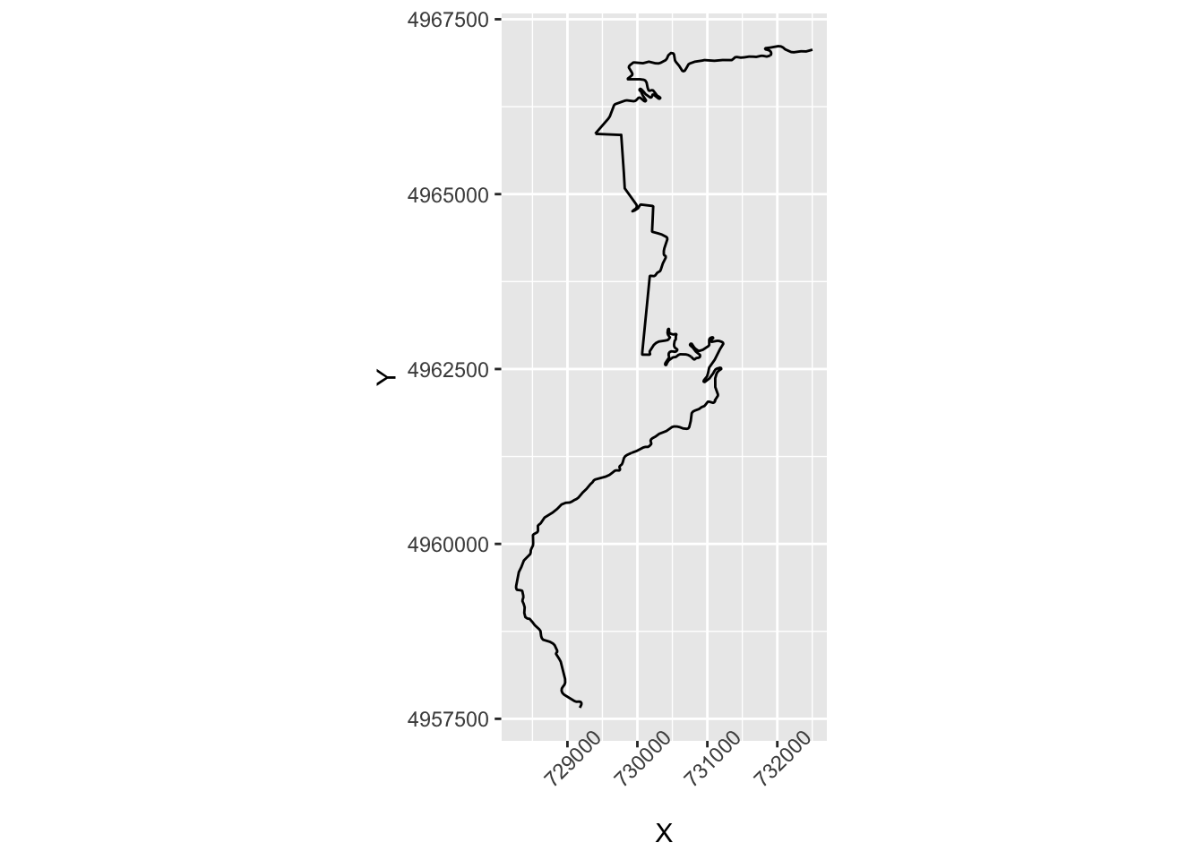

Does that shape look familiar?

If we plot the three charts side by side with a vertical alignment, we see how the “geo sensitive” plot and the UTM plot roughly correspond to each other, whereas the the latlong plot is differently proportioned:

no_labels = theme(axis.text.x = element_blank(),
                  axis.text.y = element_blank())
                    
ggpubr::ggarrange(g_sf + no_labels,
                  g_ll + no_labels,
                  g_utm + no_labels,
                  ncol=3, align='v')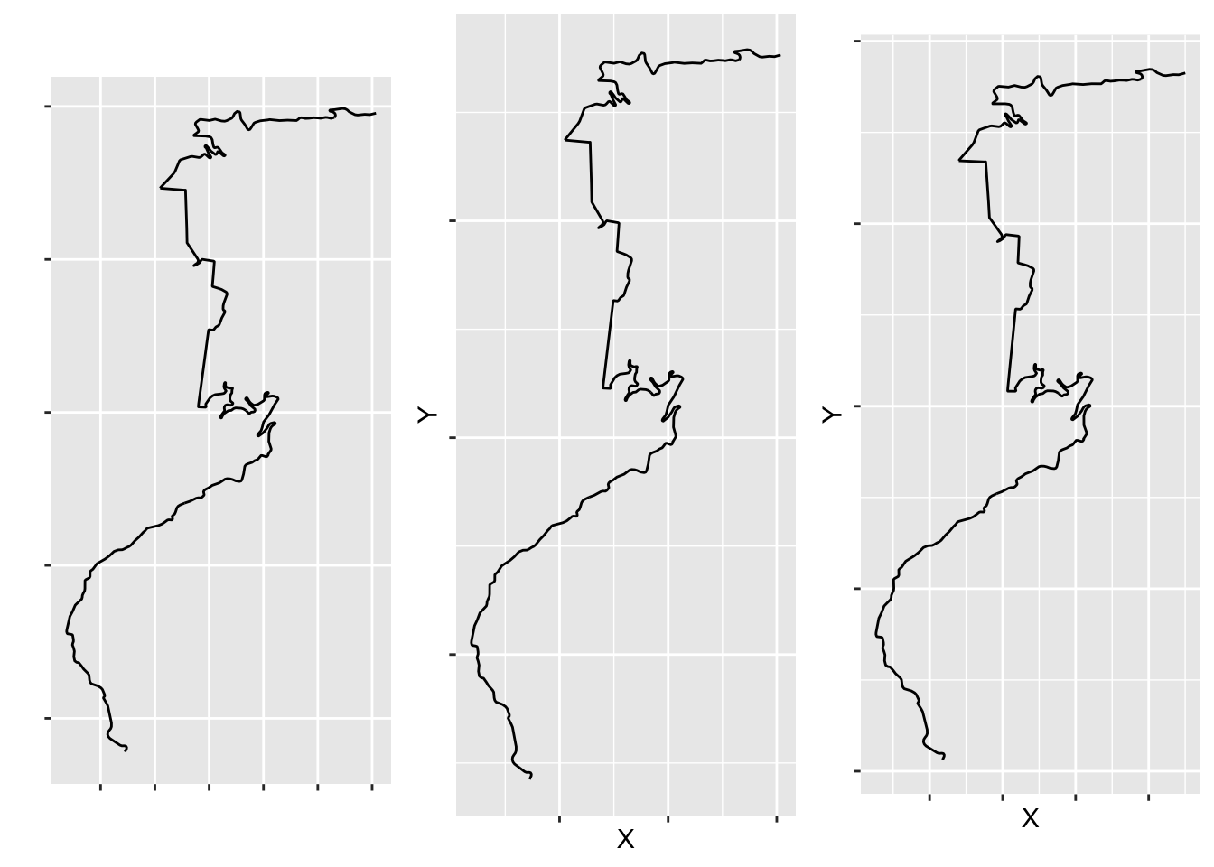

Well, it works, but it’s painful to have to go through the motions to fo it; surely there’s a better way?

5.4.2 Using ggplot2::coord_sf to Render Projections

Having the transform the coordinates from one CRS to another is a hassle; it would be so much easier if we could pass latitude and longitude coordinates into the data frame in units of degrees and let the chart map to an appropriate direction.

It so happens that we can. By setting ggplot2::coord_sf(crs), we can force the chart to use an appropriate projection:

ggplot(coords_df, aes(x=X, y=Y)) +
          geom_path() +
          coord_sf(crs=st_crs(geojson_sf[1,]))

There’s a huge range of projections available, but these two are perhaps the most convenient due to their familiarity and widespread use.

5.4.3 Exporting the Route Data As a Dataframe

For convenience, it may be useful to export the route data as a dataframe that includes both the latlong and the UTM coordinates. However, taking such a route would require creating an appropriate dataframe format for writing to a CSV file, for example, as well as means of parsing the data back in in an appropriate way.

5.5 Alternative CRS Projections

At times, finding the correct UTM zone can be a faff. In such cases, it may be convenient to use an Azimuthal equidistant (AEQD) projection: sf::st_transform(route, crs="+proj=aeqd").

For more discussion about selecting projections, see for example Geographic projections and transformations: which projection to use? (Robin Lovelace) and Geographic vs projected coordinate reference systems (Python code examples).