18 Elevation Data Revisited

Having access to elevation data is essential for rendering 3D terrain maps. But we can also plot elevation data along a single dimension: the distance along route.

For winter mountain rallies, such as Monte Carlo, elevation data may be important when estimating temperature drops along a stage caused by elevation changes, and hence the likelihood, or otherwise, of snow. (Shadow models and the time of day a stage is running, as well as the weather conditions, may also play into that).

When planning hill climbs, or rally stages that perhaps involve electric vehicle competitors, a good understanding of elevation changes, and potential energy requirements resulting from climbs, may also be important,

Rally Maps routes come with elevation profiles of this sort, and stage reports for major cycling races such as le Tour de France are rarely complete with a stage elevation maps show the cols to be encountered along the route. The cyclingcols.com website demonstrates several interesting ways of analysing cycling cols.

So can we produce our own elevation profiles from the stage route and elevation data? We surely can…

Elevation along route profiles are extracted from an elevation raster. Note that we can also extract shadow along route information from a shade raster generated for a particular data and time of day.

18.1 Load in Base Data

As ever, let’s load in our stage data and the elevation raster and create a demo map:

library(sf)
library(raster)
library(rayshader)

geojson_filename = 'montecarlo_2021.geojson'
geojson_sf = sf::st_read(geojson_filename)

## Reading layer `montecarlo_2021' from data source `/Users/tonyhirst/Documents/GitHub/visualising-rally-stages/montecarlo_2021.geojson' using driver `GeoJSON'
## Simple feature collection with 9 features and 2 fields
## geometry type:  LINESTRING
## dimension:      XY
## bbox:           xmin: 5.243488 ymin: 43.87633 xmax: 6.951953 ymax: 44.81973
## geographic CRS: WGS 84

stage_route_gj = geojsonio::geojson_json(geojson_sf[1,]$geometry)

# Previously downloaded buffered TIF digital elevation model (DEM) file
stage_tif = "buffered_stage_elevation.tif"

# Load in the previously saved image raster
elev_img = raster(stage_tif)

# Note we can pass in a file name or a raster object
elmat = raster_to_matrix(stage_tif)

## [1] "Dimensions of matrix are: 468x626."

demo_map = elmat %>%
              sphere_shade(texture = "desert", progbar = FALSE)

18.2 Generating Elevation Maps

With the geo data provided for the stage route, we only have access to the latitude and longitude of each point along the route, not the elevation.

We have already seen how we can create a route layer that we can overlay on the 3D model, with the elevation then inferred so that the route is plotted correctly on the 3D rendered model. But can we access the actual elevation values along the route somehow?

18.2.1 Accessing Elevation Values Along a Route from an Elevation Raster

The elevation raster provides an elevation value for each pixel in the raster image. We can transect the raster with a route to get the elevation value for each point along the route.

To get a routepoints list, we can extract the coordinates from a linestring geometry, casting the result to a dataframe and then selecting just the X (longitude) and Y (latitude) values:

routepoints = subset(as.data.frame(st_coordinates(geojson_sf[1,])),
                     select = c('X', 'Y'))
head(routepoints)

##          X        Y
## 1 5.894486 44.73562
## 2 5.894618 44.73580
## 3 5.894778 44.73602
## 4 5.894805 44.73621
## 5 5.894672 44.73636
## 6 5.894407 44.73642

We can add a Z (elevation) column to the dataframe by extracting the elevation at each point (that is, for each row of the dataframe) from the elevation raster image:

routepoints$elevation = raster::extract(elev_img, routepoints)
head(routepoints)

##          X        Y elevation
## 1 5.894486 44.73562      1035
## 2 5.894618 44.73580      1033
## 3 5.894778 44.73602      1032
## 4 5.894805 44.73621      1033
## 5 5.894672 44.73636      1033
## 6 5.894407 44.73642      1034

Finding the minimum and and maximum altitude along the route is trivial:

c(max(routepoints$elevation, na.rm=T), min(routepoints$elevation, na.rm=T))

## [1] 1036  769

18.2.2 Using geosphere::distGeo to Find Distance Along a Route

We can use the geosphere::distGeo() function to calculate distance in meters between each point under the WGS84 projection without having to first convert to a projection with units of meters.

The function returns the distance between consecutive locations, with a null value returned for the final step. If we want to back refer distances — how far since the last point, rather than how far to the next point — we can drop the last NA distance and prepend a distance of 0 to the start of the list of distances:

stage_coords = st_coordinates(geojson_sf[1,])[,c('X','Y')]
stage_step_distances = geosphere::distGeo(stage_coords)

# The last step distance is NA, so drop it
# Also prepend the distances with 0 for the first step
routepoints$gs_dist = c(0, head(stage_step_distances,-1))
routepoints$gs_cum_dist = cumsum(routepoints$gs_dist)

head(routepoints)

##          X        Y elevation  gs_dist gs_cum_dist
## 1 5.894486 44.73562      1035  0.00000     0.00000
## 2 5.894618 44.73580      1033 22.57054    22.57054
## 3 5.894778 44.73602      1032 27.93282    50.50337
## 4 5.894805 44.73621      1033 21.00098    71.50435
## 5 5.894672 44.73636      1033 20.38067    91.88502
## 6 5.894407 44.73642      1034 21.77090   113.65592

We can now preview the elevation against the distance along the route:

library(ggplot2)

ggplot(routepoints, aes(x=gs_cum_dist, y=elevation)) + geom_line()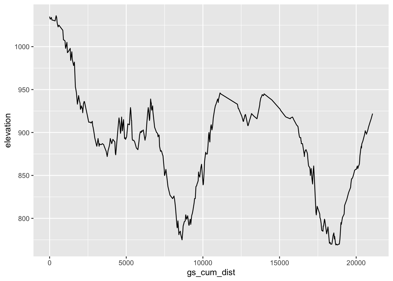

18.2.3 Using sp::spDists to Find Distance Along a Route

The sp::spDists function also allows us to find the distance between Spatial point WPS84 / longlat projected points in meters without first having to convert the points to a projection with units of meters. The function returns the “step” distance as well as the accumulated distance:

# Find the distance between points in two lists of coordinates
distances = sp::spDists(rbind(stage_coords[1,], stage_coords),
                        stage_coords,
                        longlat = TRUE)

# Extract the step and accumulated distances in km
# and convert to meters
routepoints['sp_cum_dist'] = distances[1,] * 1000
routepoints['sp_dist'] = distances[2,] * 1000

head(routepoints)

##          X        Y elevation  gs_dist gs_cum_dist sp_cum_dist  sp_dist
## 1 5.894486 44.73562      1035  0.00000     0.00000     0.00000  0.00000
## 2 5.894618 44.73580      1033 22.57054    22.57054    22.57069 22.57069
## 3 5.894778 44.73602      1032 27.93282    50.50337    50.50298 50.50298
## 4 5.894805 44.73621      1033 21.00098    71.50435    70.47300 70.47300
## 5 5.894672 44.73636      1033 20.38067    91.88502    84.52844 84.52844
## 6 5.894407 44.73642      1034 21.77090   113.65592    89.23297 89.23297

Note that the actual distances calculated vary slightly depending on the internals and settings used in the function used to calculate them. The numbers are close enough for storytelling!

18.3 Generating a 3D Ribbon Plot of the Stage Route

A ggplot2::geom_ribbon() plot provides a familiar way of rendering the elevation plot in the form a line chart with a fill that extends down to the x-axis:

library(ggplot2)

# Find a nice minimum elevation
min_elevation = max(0, 100*round(((min(routepoints$elevation)/100)-1.6)))
max_elevation = max(routepoints$elevation)

g = ggplot(routepoints, aes(x = gs_cum_dist)) +
      geom_ribbon(aes(ymin = min_elevation,
                      ymax = elevation),
                  fill = "#1B9E77") + 
      labs(x = "kilometers", y = "Elevation") +
      scale_y_continuous(limits = c(min_elevation, max_elevation))

g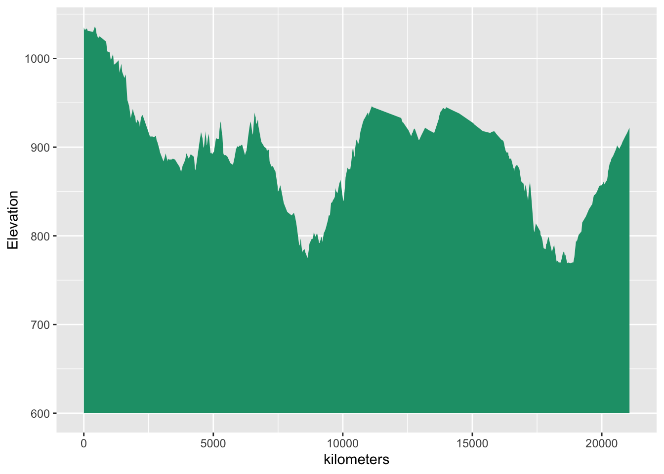

We can get a 3D plot from the ribbon chart via the rayshader::plot_gg() function:

options(rgl.useNULL = TRUE,
        rgl.printRglwidget = TRUE)

rgl::clear3d()
plot_gg(g, height=5, width=6, scale=500, raytrace=FALSE)

rgl::rglwidget()

18.4 Identifying Road Type

The OSM highways data often includes information about road class. We can use this information to add an aesthetic to the line that distinguishes the road class along the route, either by color or by width.

#Precautionary measure to clean the data
routepoints = routepoints %>% tidyr::drop_na('elevation')

# Create a min colour value 10% of the max-min range below the min value
min_val = min(routepoints$elevation) - 0.1 * (max(routepoints$elevation) -  min(routepoints$elevation))

We can use the ggplot2::coord_sf(crs=st_crs(geojson_sf)) function to allow us to a non-spatial dataframe containing latitude and longitude coordinates in a spatial way:

# We need to use the geom_path to render the route
# geom_line will plot against ordered, not consecutive, x and y
g2 = ggplot(routepoints, aes(x=X, y=Y, color=elevation))+
  geom_point(size=3) +
  geom_path(size=3.5) +
  
  # Set the coordinate system to the original projection
  coord_sf(crs=st_crs(geojson_sf)) +
  
  lims(color=c(min_val, max(routepoints$elevation)))

g2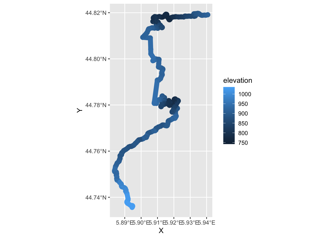

It might also be interesting to explore a line width setting to reflect the likely width of the road. For example, we might image A roads to nominally have a width of 8m, enough for two cars to pass one another, B class roads to have a width of 6m (a close squeeze) and C roads or other tracks to have a width of 4m (single track road).

18.5 Displaying Route Twistiness and Elevation

The 3D rendered ribbon chart is amusing, but not necessarily very informative. What would be far more compelling would be if we could render elevation and also the twists and turns take by the route.

So let’s do that in the form of a plot of elevation against latitude and longitude:

rgl::clear3d()

gg = plot_gg(g2, height=5, width=6, scale=500,
             raytrace=FALSE)

r = rgl::rglwidget()

widget_fn = 'elev_model.html'
htmlwidgets::saveWidget(r, widget_fn)

Embed the HTML back in an iframe:

htmltools::includeHTML(widget_fn)

18.5.1 Making a 3D Print File of the Model

As well as making movies of the stage route it is also worth reminding ourselves that we can also export the model as a 3D printer ready model. The rayshader::save_3dprint() function will export an .stl format model file directly from our model:

# We can also save the file to a 3d print stl file
model_fn = "stage_3d.stl"
save_3dprint(model_fn, maxwidth = 10, unit = "in")

## Dimensions of model are: 10.00 in x 8.33 in x 3.34 in

With model file in hand,it can then be uploaded to 3D print on demand service such as 3dpeople, 3d print UK, MakeitQuick Manufacturing or Champion 3D to provide us with a physical model of a stage.

18.5.2 Rendering a 3D movie of the Model

Render a 3D movie to provide a rotating view of the 3D rendered line char showing the route path and elevation:

library(av)

options(rgl.useNULL = FALSE,
        rgl.printRglwidget = FALSE)

rgl::rgl.open()
rgl::clear3d()

g = plot_gg(g2 + theme(legend.position = "none"),
            height=5, width=6, scale=500,
            raytrace=FALSE)

# 3D movie
video_fn = 'demo_stage_line.mp4'

#render_movie(video_fn, progbar=FALSE)
rgl::rgl.close()

embedr::embed_video(video_fn, type ="mp4",
                    width = "256", height = "256")

18.6 Using the slopes Package to Analyse Stage Elevation Data

Having got the elevation profile as elevation by distance into stage, we can borrow some ideas from the chapter on route profiling to try to identify certain features in the route, for example in terms of gradient or even “elevation-twistiness” of a climb / descent.

The slopes R package simplifies obtaining elevation data considerably, and provides an easy way to visualise slopes and steepness as well as packaging various functions relate to the ones we developed in the previous sections.

For example, the slopes::slope_3d() function takes a route linestring and a raster and adds the elevation as the Z coordinate to the linestring:

library(slopes)

route_slope_elevation = slope_3d(geojson_sf[1,], elev_img)

There is also automated support for finding elevation data from a route by omitting the raster data when calling the slopes::slope_3d() function with just the linestring.

The slopes::plot_slope() function visualises the gradient at each step along the 3D linestring route using base graphics:

plot_slope(route_slope_elevation)

Within the slopes package are several utility function for extracting step distance, elevation and gradient along the route:

route_coords = sf::st_coordinates(geojson_sf[1,])
# lonlat: is the order lonlat?
d = sequential_dist(route_coords, lonlat = TRUE)

## Loading required namespace: geodist

We can get the elevation for each line segment in the linestring using the slopes::elevation_extract() function:

e = elevation_extract(route_coords, elev_img)

Simple plot:

slopes_df = data.frame(d=c(0,d), e=e)

# Find the accumulated distanced over route steps
slopes_df$cum_d = cumsum(slopes_df$d)

ggplot(slopes_df)+geom_line(aes(x=cum_d, y=e))

We can get slope associated with each line segment using the slopes::slope_distance() function, or from the 3D linestring using the slopes::slope_matrix() function. (The lonlat parameter flags the order of longitude and latitude values.)

step_gradients = slope_distance(d, e) # d is 1 item shorter than e
step_gradients2 = slope_matrix(st_coordinates(route_slope_elevation),
                               lonlat = TRUE)

18.7 Analysing Route Elevation from First Principles

The simplest thing to calculate is probably gradient, which tells us how steep an incline / descent is at any part of the stage, as well as as where the turning points (in gradient terms) are: crests and plateaus, for example.

ggplot(routepoints, aes(x=gs_cum_dist)) + geom_line(aes( y=elevation)) +
  geom_line(aes( y=1000*pracma::gradient(elevation, gs_cum_dist)), color='red')

Areas where the gradient is greater than show the route is climbing; where the gradient is less than one shows a descent. A gradient near zero is on the flat.

We might get a slightly cleaner trace if we smooth the elevation profile and then find its gradient.

trj <- TrajFromCoords(routepoints[,c('gs_cum_dist', 'elevation')])
smoothed <- trajr::TrajSmoothSG(trj, p=3, n=9)

smoothed['y_gradient'] = 1000*pracma::gradient(smoothed$y,smoothed$x)
ggplot()+geom_line(data=routepoints,aes(x=gs_cum_dist, y=elevation)) +geom_line(data=smoothed, aes(x=x, y=y), color='red') +
  geom_line(data=smoothed, aes(x=x, y=y_gradient), color='blue')

Another technique we might use to display the data is to create coloured bands, as per a ribbon plot, coloured according to the whether the gradient is positive or negative, using the magnitude of the gradient to set the colour intensity as per a heat map.

smoothed$col[smoothed$y_gradient >= 0] <- "climbing"
smoothed$col[smoothed$y_gradient < 0] <- "descending"

# Doing something wrong with the fills here?
ggplot(smoothed, aes(x=x, y=y_gradient)) +
  geom_area(aes(fill=col)) +
  geom_line() +
  geom_hline(yintercept=0)

# geom_ribbon has the same issue