An Aside - The Penny Red

Although our main focus in using rayshader’s 3D plotting capabilities will be to render 3D interactive maps, it’s worth bearing in mind that rayshader can be used as a general purpose 3D visualisation tool.

So before we start rendering 3D maps, and before we are tempted to think that maps are the only thing we can plot with rayshader, let’s visualise something completely different: the colour of a Penny Red stamp…

We can obtain an appropriate image file from Wikipedia and save a local copy of it:

image.url = 'https://upload.wikimedia.org/wikipedia/commons/a/a4/PennyRed.jpeg'
pennyred_file = 'PennyRed.jpeg'

# Download the file from a specified web location to a specifically named file
download.file(image.url, pennyred_file)

3D Rendering of Colour Images Using rayshader

To use rayshader to render the image file, we need to obtain some “elevation” levels that will project some attribute of the image into the vertical z dimension.

One obvious candidate is the RGB colour value (we might alternatively render just the red, green or blue components) mapped to a single elevation value by regarding it as a base 256 encoded value:

library(raster)

pennyred_image =  jpeg::readJPEG(pennyred_file)
# Also:  png::readPNG(png_file)

# Create a raster file from the image
pennyred = raster(pennyred_file)

# Isolate the reg, green and blue components
pennyred_red = pennyred_image[,,1]
pennyred_green = pennyred_image[,,2]
pennyred_blue = pennyred_image[,,3]

#https://www.maptiler.com/news/2019/03/rgb-encoded-elevation-data-in-maptiler-cloud/
# height = -10000 + ((R * 256 * 256 + G * 256 + B) * 0.1)

# Use the RGB values as a base 256 elevation encoding
# then reduce the height with a base value
# We should really calculate the base value rather than use a 
# value determined by observation...
# The values() function sets the value of the pennyred raster
values(pennyred) = -16700 + (((255-pennyred_red ) * 256 * 256 +
                              (255-pennyred_green ) * 256 +
                              (255-pennyred_blue)) * 0.001)

# The pennyred raster now has values that encode RGB-as-elevation
pennyred

## class      : RasterLayer 
## band       : 1  (of  3  bands)
## dimensions : 234, 200, 46800  (nrow, ncol, ncell)
## resolution : 1, 1  (x, y)
## extent     : 0, 200, 0, 234  (xmin, xmax, ymin, ymax)
## crs        : NA 
## source     : memory
## names      : PennyRed 
## values     : 11.42209, 58.69265  (min, max)

To create an elevation matrix from the data, we might consider scaling from the raw RGB values:

elev_matrix_pennyred <- matrix(
      raster::extract(pennyred, raster::extent(pennyred)), 
      nrow = ncol(pennyred), ncol = nrow(pennyred)
)

The rayshader package takes a simple elevation matrix and renders it in 2 or 3 dimensional relief.

For example, here’s a simple 2D rendering:

library(rayshader)

elev_matrix_pennyred %>%
  sphere_shade(texture = "desert") %>%
  #add_overlay(pennyred_image) %>%
  plot_map()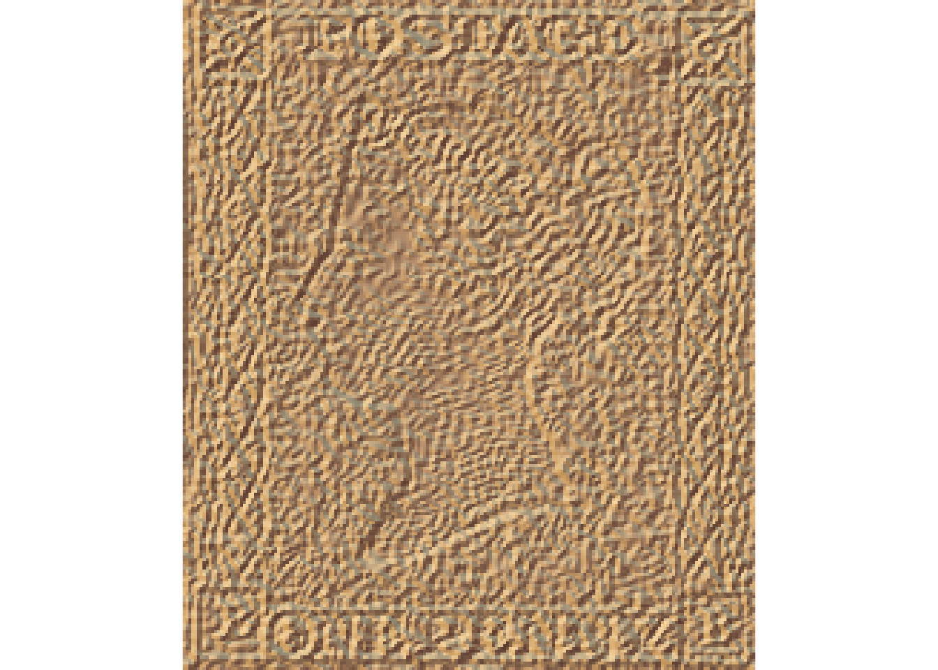

  #plot_3d(elev_matrix_pennyred)

We can also add the original image back as an overlay. In this case, we lose the 3D effect:

rayshaded_penny_red = elev_matrix_pennyred %>%
  sphere_shade(texture = "desert") %>%
  add_overlay(pennyred_image)

rayshaded_penny_red %>%
  plot_map()

However, if we view the elevated image in a 3D plot, we can see the elevation map far more clearly:

# Configuration settings to allow us to render the WebGL 
options(rgl.useNULL = TRUE,
        rgl.printRglwidget = TRUE)

rgl::clear3d()

rayshaded_penny_red %>%
  plot_3d(elev_matrix_pennyred)

rgl::rglwidget()

# knitr widget embed example via:
# https://github.com/Robinlovelace/geocompr/blob/master/08-mapping.Rmd
# maybe set options?
#knitr::opts_chunk$set(widgetframe_widgets_dir = 'widgets' )
# Save widget to a local file
# w_file = "penny_red_3d_widget.html"
# htmlwidgets::saveWidget(r, w_file)
# We then need to save the file to a URL to use:
# knitr::include_url(URL)
# Or just explicitly use an iframe to load the local file?

11.5.1 Rendering the image directly from ggplot2

Whilst we can try to work out our own method for creating elevation models from an image, its much easier to use another tool that rayshader provides: the plot_gg() function.

This function can render a 3D plot directly from a ggplot2 object using the color or fill aesthetic for the elevation values. All the mappings from color to elevation are handled automatically, as is the overlaying of the original image.

So how do we get an image into a ggplot2 object?

The imager R package contains some handy utilities for working with images further.

For example, it allows is to straightforwardly plot an image loaded in directly from a file:

i_imager <- imager::load.image(pennyred_file)
plot(i_imager)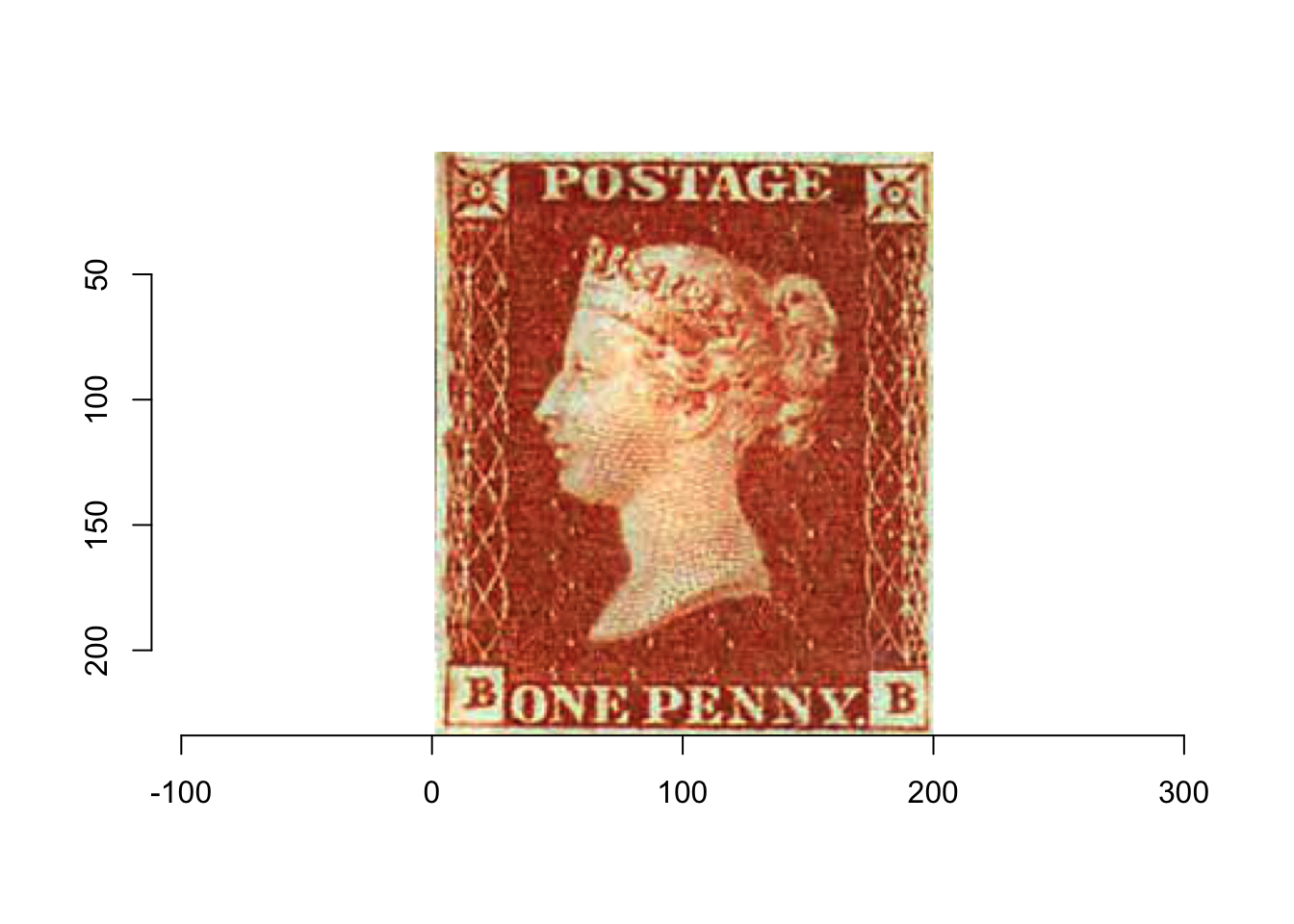

We can cast the image as a dataframe, where each row contains an x and a y co=ordinate, the colour channel, cc and the color value:

i_df <- as.data.frame(i_imager)

head(i_df)

##   x y cc     value
## 1 1 1  1 0.8901961
## 2 2 1  1 0.8156863
## 3 3 1  1 0.7803922
## 4 4 1  1 0.7019608
## 5 5 1  1 0.7176471
## 6 6 1  1 0.7960784

With the data in a data frame form, we can the plot from it using ggplot() in the normal way:

library(ggplot2)

df <- imager::grayscale(i_imager) %>% as.data.frame

gg_pr = ggplot(df,aes(x,y)) + geom_raster(aes(fill=value)) +
  scale_y_continuous(trans=scales::reverse_trans()) +
  scale_fill_gradient(low="black",high="white") +
  coord_fixed()

gg_pr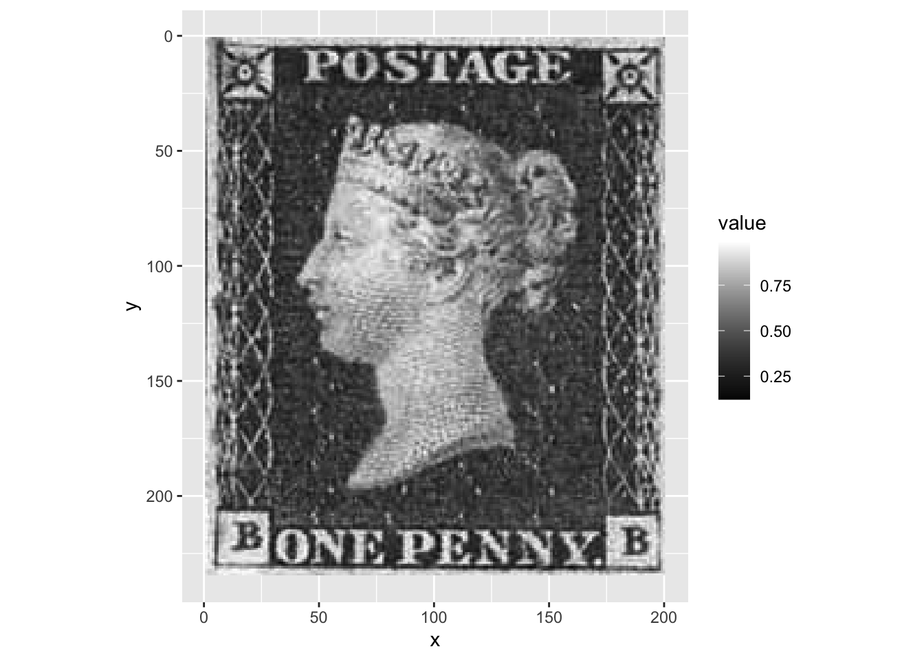

How about if we pass a full colour image to the ggplot()?

library(dplyr) # for mutate

df2 <- as.data.frame(i_imager, wide="c") %>% 
  mutate(rgb.val=rgb(c.1,c.2,c.3))

gg_pr2 = ggplot(df2, aes(x,y)) +
  geom_raster(aes(fill=rgb.val)) +
  scale_fill_identity() +
  coord_fixed() +
  scale_y_continuous(trans=scales::reverse_trans())

gg_pr2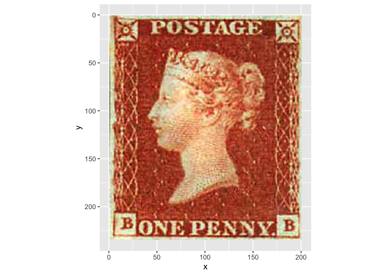

Rendering a Movie

How can we best show off the 3d rendering of the elevated image? One way is to plot the ggplot() image as a 3D model using the rayshader::plot_gg() function and then render a movie from it using a custom shooting script to drive the camera:

# Configuration settings to allow us to render the movie
options(rgl.useNULL = FALSE,
        rgl.printRglwidget = FALSE)

library(av)

rgl::rgl.open()
rgl::clear3d()

#Create the plot
plot_gg(gg_pr2, width=5, height=5, scale=250,
        raytrace = FALSE)

# Interesting camera orbit for previewing 3d plots from ggplot

# Script from https://joeystanley.com/blog/3d-vowel-plots-with-rayshader
# which seems to have pinched it form a tutorial somewhere?
#render_movie('demo_pennyred.mp4')

# Set up the camera position and angle
phivechalf = 30 + 60 * 1/(1 + exp(seq(-7, 20, length.out = 180)/2))
phivecfull = c(phivechalf, rev(phivechalf))
thetavec = 0 + 60 * sin(seq(0,359,length.out = 360) * pi/180)
zoomvec = 0.45 + 0.2 * 1/(1 + exp(seq(-5, 20, length.out = 180)))
zoomvecfull = c(zoomvec, rev(zoomvec))


# 3D movie
video_fn = 'demo_pennyred.mp4'

# Actually render the video.
#render_movie(filename = video_fn, type = "custom", 
#            frames = 360, zoom = zoomvecfull,
#            phi = phivecfull, theta = thetavec)

rgl::rgl.close()

embedr::embed_video(video_fn, width = "256", height = "256")

So with that taste of what rayshader can do, let’s get back to our rally data…