11 Annotating `rayshader` maps

As well as adding computed shading, contour and water overlays to maps, we can also enrich rayshader maps with additional annotations such as title information, or, of

11.1 Load in Base Data

As ever, let’s load in our stage data and the elevation raster and create a demo map:

geojson_filename = 'montecarlo_2021.geojson'
geojson_sf = sf::st_read(geojson_filename)

## Reading layer `montecarlo_2021' from data source `/Users/tonyhirst/Documents/GitHub/visualising-rally-stages/montecarlo_2021.geojson' using driver `GeoJSON'
## Simple feature collection with 9 features and 2 fields
## geometry type:  LINESTRING
## dimension:      XY
## bbox:           xmin: 5.243488 ymin: 43.87633 xmax: 6.951953 ymax: 44.81973
## geographic CRS: WGS 84

library(raster)
library(rayshader)

# Previously downloaded TIF digital elevation model (DEM) file
stage_tif = "stage_elevation.tif"

# Load in the previously saved image raster
elev_img = raster(stage_tif)

# Note we can pass in a file name or a raster object
elmat = raster_to_matrix(stage_tif)

demo_map = elmat %>%
              sphere_shade(texture = "desert")

11.2 Adding a Title to a Map

We can add a title to the image as a layer using the rayimage::add_title() function [docs].

Currently, the title is overlaid on top of the image, so we would need to add a buffer to account for the area taken up by the label if we didn’t want to occlude anything in the image by the title. (Can we calculate how much vertical padding is required?)

demo_map %>%
  rayimage::add_title("Stage Map", title_size = 20, 
                      title_bar_color = "red",
                      title_bar_alpha=0.8,
                      title_color="white",
                      title_offset = c(120,12), #offset from top left
                      title_style='italic',
                      #title_position='south', # But doesn't relocate bar?
                      ) %>%
  plot_map()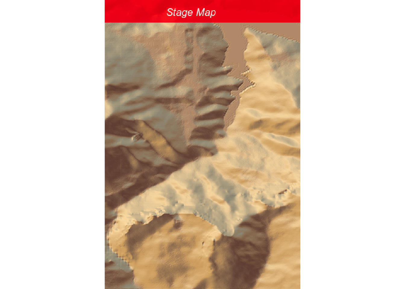

Another way of using this feature might be to set the transparency level and show stage results, or example, overlaid on the stage map whilst also seeing the map below.

It would be useful if we could set the width and location of the title and title_bar [issue].

The title and title bar can also be added (with similar arguments as to rayimage::add_title()) via the plot_map() function:

demo_map %>%
  plot_map(title_text='Stage Map',
           title_size = 20,
           title_bar_color = "red",
           title_bar_alpha=0.8,
           title_color="white",
           title_offset = c(120,12), #offset from top left
           title_style='italic',
           #title_position='south', # But doesn't relocate bar?)
  )

11.3 Adding Contours to `rayshader` Stage Maps

We have already seen how we can add contours to a raster image. A contour layer can also be created using the rayshader::generate_contour_overlay() function:

contour_color = "#ffffff" #"#7d4911"

contours_layer = generate_contour_overlay(elmat, color = contour_color, 
                                       linewidth = 1, 
                                       levels=seq(min(elmat),
                                                  max(elmat),
                                                  by=20))
# Increasing the by argument separates out lines;
# This may be important for seeing steep inclines

We can then add the overlay in the normal way:

contoured_map = demo_map %>% 
                  add_overlay(contours_layer,
                              alphalayer = 0.9)

contoured_map %>%  
   plot_map()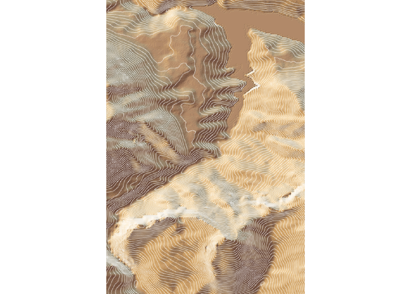

11.4 Overlaying Image Tiles

As well as creating out own shaded terrain over the raster, we can also overlay tiles retrieved from a 2D map tile server:

overlay_image_terrain <-
  geoviz::slippy_overlay(elev_img, 
                 image_source = "stamen",
                 image_type = "terrain",
                 png_opacity = 0.9)

demo_map %>% 
  add_overlay(overlay_image_terrain) %>%
  plot_map()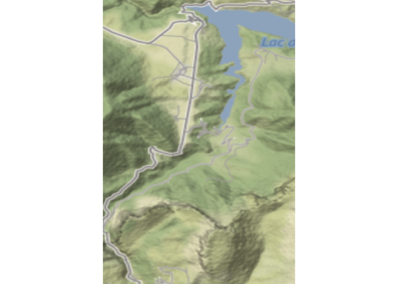

11.5 Plotting Route Layers on `rayshader` Maps

As well as previewing the OSM retrieved roads within the bounding box area of a stage route and the stage routes themselves using simple a ggplot2 view, we can also render roads and stage routes as layers on a rayshader map.

Let’s start by creating a line overlay containing the roads in the rendered area:

library(osmdata)

stage_osm  = opq(sf::st_bbox(geojson_sf[1,])) %>% 
  add_osm_feature("highway") %>% 
  osmdata_sf()

stage_lines = stage_osm$osm_lines

stage_roads = stage_lines[stage_lines$highway %in% c("unclassified", "secondary", "tertiary", "residential", "service"), ] 


roads_layer = generate_line_overlay(stage_roads,
                                    extent = extent(elev_img),
                                    color="yellow",
                                    heightmap = elmat)

We can also create a layer that identifies the stage route, colouring it and setting the line width as required to make it stand out in the rendered view.

In the following example, we create a red coloured stage route layer:

red_route = generate_line_overlay(geojson_sf[1,],
                                    extent = extent(elev_img),
                                    heightmap = elmat,
                                    linewidth = 5, color="red")

We can now add the roads and stage overlays to our map:

demo_map %>%
  add_overlay(roads_layer)  %>%
  add_overlay(red_route) %>%
  plot_map()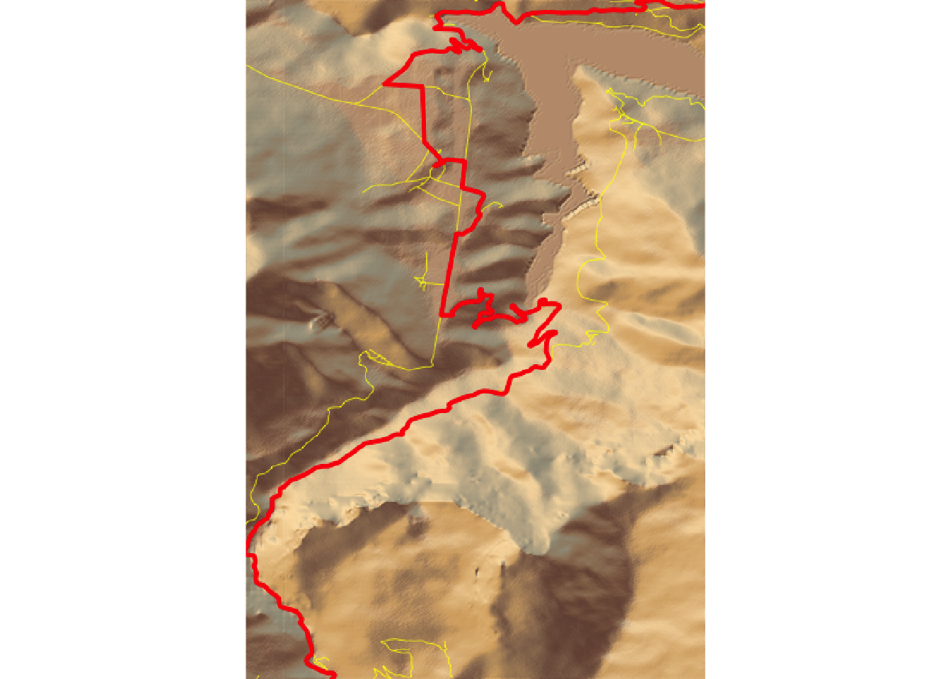

This may not look so interesting in a 2D view, but as you will seem it does provide a way of bringing the tile to life when we look at in as an interactive 3D view of 3D video view…

11 Annotating rayshader maps