16 Composing rayshader Stills and Movies
If we have access to a desktop rgl renderer, we can easily generate snapshots and movies of our rendered scenes. Without the desktop rendering, things are slower.
Such is the way of things, I left the arty 3D rendering sections to do till last, and in the three weeks since I started playing with rayshader, then parked it as I moved on to other chapters, many things rendering now seem differently broken to me. I updated something and can’t find any version combinations of packages that get me back to where I was. Should’a baked it into a Docker container… :-( So this is something I’ll have to return to at some point to see if things have started working again. Ho hum…
16.1 Load in Base Data
As ever, let’s load in our stage data:
geojson_filename = 'montecarlo_2021.geojson'
geojson_sf = sf::st_read(geojson_filename)## Reading layer `montecarlo_2021' from data source `/Users/tonyhirst/Documents/GitHub/visualising-rally-stages/montecarlo_2021.geojson' using driver `GeoJSON'
## Simple feature collection with 9 features and 2 fields
## geometry type: LINESTRING
## dimension: XY
## bbox: xmin: 5.243488 ymin: 43.87633 xmax: 6.951953 ymax: 44.81973
## geographic CRS: WGS 84And also load in the elevation data raster:
library(raster)
library(rayshader)
# Previously downloaded TIF digital elevation model (DEM) file
stage_tif = "buffered_stage_elevation.tif"
# Load in the previously saved image raster
elev_img = raster(stage_tif)
auto_zscale = geoviz::raster_zscale(elev_img)
# Note we can pass in a file name or a raster object
elmat = raster_to_matrix(stage_tif)Let’s create a demo map that we can use as as test piece:
demo_map = elmat %>%
sphere_shade(texture = "desert") %>%
add_water(detect_water(elmat, progbar = FALSE),
color = "desert")We need to ensure we are rendering into a desktop rgl canvas, rather than a WebGL widget:
But that’s all broken for me atm, making this a TO DO item. OpenGL not compiled in to the package I’m using and I can’t find an old version that works the way it used to for me…
options(rgl.useNULL = FALSE,
rgl.printRglwidget = FALSE)16.1.0.1 Creating Titles and Overlays
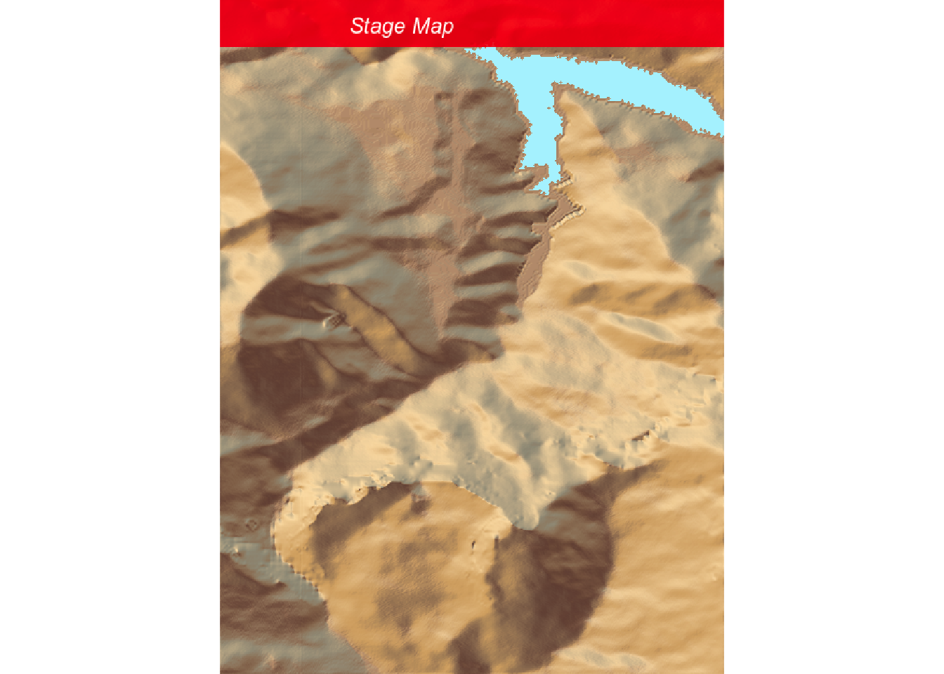
The rayshader::plot_map() functions allow us to add a title to a view. The title text sits on top a coloured title bar, with configurable colour and transparency.
The title text can be repositioned using the title_position attribute but the title bar doesn’t seem to be transported with it…
demo_map %>%
plot_map(title_text='Stage Map',
title_size = 20,
title_bar_color = "red",
title_bar_alpha=0.8,
title_color="white",
title_offset = c(120,12), #offset from top left
title_style='italic',
#title_position='south', # But doesn't relocate bar?)
)
We can also add titles to rendered 3D views with the rayshader::render_snapshot() function:
rgl::clear3d()
demo_map %>%
plot_3d(elmat, zscale = auto_zscale)
title_fn = "demo_stage_3D_title_overlay.png"
render_snapshot(title_fn,
title_text='Stage Map',
title_size = 20,
title_bar_color = "red",
title_bar_alpha=0.8,
title_color="white",
title_offset = c(120,12), #offset from top left
title_style='italic',
#title_position='south', # But doesn't relocate bar?)
)
knitr::include_graphics(title_fn)
We can also add an image overlay with the image_overlay attribute set to the path of a png image file (with transparency) or a 4-layer RGBA array. The image will be resized to the dimension of the image if the dimensions don’t match and overlaid on the original.
It might be useful to create a function that can take a smaller image, such as a stage results table, and buffer it with a transparent margin to match the raster size?
16.1.1 Adding Complications…
We can add watchmaker style complications to the chart in the form of a scalebar and a compass to show the direction:
rgl::clear3d()
demo_map %>%
plot_3d(elmat, zscale=auto_zscale)
render_scalebar(limits=c(0, 5, 10),label_unit = "km",
position = "S", y=50,
scale_length = c(0.33, 1))
render_compass(position = "E")
complications_fn = "demo_stage_3D_map_complications.png"
render_snapshot(complications_fn)
knitr::include_graphics(complications_fn)
16.2 Setting Up the Camera Shots in rayshader
This is just to slow TO DO when we have to work with webshot2. Revisit another day, hopefully…:-(
A wide variety of controls and functions are available that allow us to use rayshader as a virtual studio for capturing views of the landscape from arbitrary positions and with a wide variety of camera and lighting settings.
16.2.1 Depth of Field
The rayshader::render_depth() function gives us control over the depth of field and provides all sort of parameters that folk who like twiddling things on their camera might enjoy. From the docs, the following controls are available:
- virtual camera settings:
- focus: depth in which to blur (0..1)
- focallength
- fstop
- bokeh settings:
- bokehshape: circle or hex
- rotation: number of degrees to rotate the hexagon bokeh shape
- bokehintensity: intensity of the bokeh when the pixel intensity is greater than ‘bokehlimit’
- bokehlimit: limit after which the bokeh intensity is increased by ‘bokehintensity’
- image manipulation:
- gamma_correction: control gamma correction when adding colors
- aberration: add chromatic aberration to the image.
A preview_focus flag is also provided that can be used to display a red line across the image showing where the camera will be focused.
Let’s generate a gallery of some possible settings:
rgl::clear3d()
demo_map %>% plot_3d(elmat, zscale=auto_zscale)
render_depth(focus = 0.81, focallength = 200,
title_bar_color = "black",
vignette = TRUE,
title_text = "SS1, Rallye Monte Carlo, 2021",
title_color = "white", title_size = 50)
test_fn = 'test8.png'
render_snapshot(test_fn)
knitr::include_graphics(test_fn)TO DO - maybe generate an animated gif showing various settings?
16.3 Camera Positioning
As well as generating “quick” rendered snapshots of a scene using the rayshader::render_snapshot() function, we can also set up a scene and render it using the rayshader:render_highquality() function.
The rayshader::render_highquality() function combines the ability to render a scene with camera positioning, title adding and other scene management controls.
For example, we can use the rayshader::render_camera() function to position the camera and set various camera properties:
- theta: rotation of the model in the xy-plane
- phi: azimuth angle, height above the horizon
- fov: field of view in degrees (maximum 180)
- zoom: magnification of the camera zoom (>0)
A masterclass by rayshader creator Tyler Morgan-Wall uses the following video to demonstrate the between the theta and phi settings, the camera position and the camera view:
video_url = "https://www.tylermw.com/data/all.mp4"
embedr::embed_video(video_url, type='mp4')In an RMarkdown document, we can set the camera location after generating the 3D plot, but before rendering it via the widget. We could equally render the plot to an image from that position rather then rendering the widget to view the model interactively.
TO DO - this should equally position the camera in the OpenGL window and then let us take a really quick snapshot…
rgl::clear3d()
demo_map %>% plot_3d(elmat, zscale=auto_zscale)
render_camera(theta = 40, phi = 70, zoom = 1.5, fov = 90)
rgl::rglwidget()