13 Rendering 3D rayshader Stage Route Maps

Having introduced interactive 3d rayshader models in the previous chapter, let’s now explore how we can generate interactive three dimensional models of our stage maps.

13.1 Load in Base Data

As ever, let’s load in our stage data:

library(tidyr)

geojson_filename = 'montecarlo_2021.geojson'
geojson_sf = sf::st_read(geojson_filename)

## Reading layer `montecarlo_2021' from data source `/Users/tonyhirst/Documents/GitHub/visualising-rally-stages/montecarlo_2021.geojson' using driver `GeoJSON'
## Simple feature collection with 9 features and 2 fields
## geometry type:  LINESTRING
## dimension:      XY
## bbox:           xmin: 5.243488 ymin: 43.87633 xmax: 6.951953 ymax: 44.81973
## geographic CRS: WGS 84

stage_bbox = sf::st_bbox(geojson_sf)

We have already seen how we can overlay an elevation model raster on a leaflet map, as well as rendering two dimensional topographic models using the raytracer package. Generating 3D, rather than 2D, maps follows exactly the same steps as the 2D view apart from the final rendering step.

Recall that the raytracer package itself works with a matrix of raster values. Having saved the download raster to a tif file, we can load the data back in from and convert it to a matrix using the rayshader::raster_to_matrix() function:

library(rayshader)
library(raster)

# Previously downloaded buffered TIF digital elevation model (DEM) file
stage_tif = "buffered_stage_elevation.tif"

# Load in the previously saved image raster
elev_img = raster(stage_tif)

# Get the natural zscale
auto_zscale = geoviz::raster_zscale(elev_img)

# Note we can pass in a file name or a raster object
elmat = raster_to_matrix(stage_tif) 

Just as a reminder, here’s a quick review of what the 2D maps look like:

# Use the raster extent for the plots
stage_extent = extent(elev_img)

yellow_route = generate_line_overlay(geojson_sf[1,],
                                    extent = stage_extent,
                                    heightmap = elmat,
                                    linewidth = 5, color="yellow")

mapped_route_yellow = elmat %>%
  sphere_shade(sunangle = -45, texture = "bw") %>%
  #add_water(watermap, color = "bw") %>%
  add_overlay(yellow_route)

mapped_route_yellow %>%
  plot_map()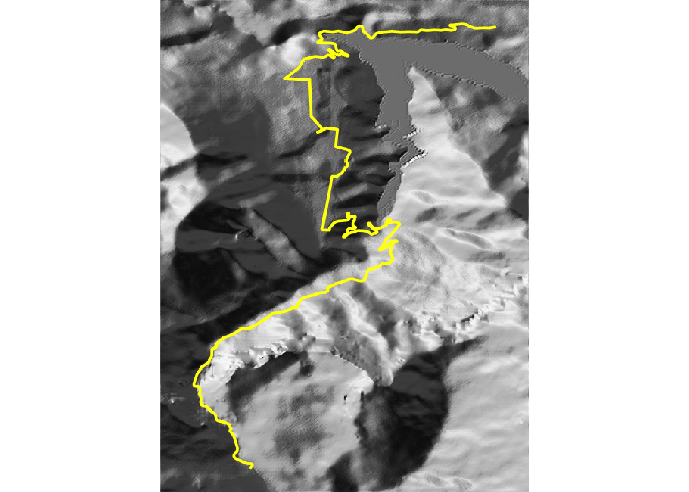

The 2D plots can be quite pretty, but we can also bring them even more alive as 3D rendered plots.

13.2 Setting Up 3D Embedded Plots

Recall that to embed WebGL interactive models using rgl::rglwidget(), we need to fettle some settings first:

options(rgl.useNULL = TRUE,
        rgl.printRglwidget = TRUE)

13.3 Rendering a Simple Stage Route Model

We can render our 2D route model simply by passing it to the rayshader::plot_3d() function, along with the elevation model.

If we set the zscale parameter to the auto_zscale determined previously as auto_zscale = geoviz::raster_zscale(elev_img), the relief is rendered using the “real” scaling that keeps the height of elevated areas in equal proportion to the scale used by the x and y scale values:

rgl::clear3d()

mapped_route_yellow %>%
  plot_3d(elmat, zscale=auto_zscale)

rgl::rglwidget()