12 Introducing 3D rayshader Models

One of the most powerful features of the rayshader package is the support if provides for generating and working with 3D rendered models of map views, providing a far more powerful toolkit than offered by tools such as rasterVis::plot3D(). In this chapter, we’ll demonstrate how to get started creating 3D rendered interactive rayshader models.

12.1 Rendering the 3D Maps in RStudio& and knitrable Rmd* Documents

The 3D map views can be rendered in a couple of ways. To create the rendering, rayshader uses the rgl package.

According to the rgl docs:

[t]here are two ways in which rgl scenes are normally displayed within R. The older one is in a dedicated window. In Unix-alikes this is an X11 window; it is a native window in Microsoft Windows. On MacOS, the XQuartz system (see https://www.xquartz.org) needs to be installed to support this. To suppress this display, set options(rgl.useNULL = TRUE) before opening a new rgl window.

This original approach requires access to an X11 style window. When using a headless environment, such as a Docker environment running RStudio via a web browser, or a MyBinder environment running Jupyter notebooks with an R kernel, the first route is unlikely to work without significant set up and configuration requirements.

The second approach, which we might consider to be the headless, web native approach, is to use WebGL:

The newer way to display a scene is by using WebGL in a browser window or in the Viewer pane in RStudio. To select this, set options(rgl.printRglwidget = TRUE). Each operation that would change the scene will return a value which triggers a new WebGL display when printed. In an R Markdown document in knitr, use the rgl::rglwidgetfunction. (You can also use chunk optionwebgl=TRUE; we recommend the explicit use of ``rglwidget.) This approach also allows display of rgl scenes in RStudio.

# Using the latest version of rgl is currently advised:
# remotes::install_github("dmurdoch/rgl")
#remotes::install_github("dmurdoch/rgl", type = 'source')

# FOllowing is currently broken for me
# install.packages("rgl", repos = "http://R-Forge.R-project.org", type = "source")
# 

Settings for running in a headless / RStudio / knitr environment:

# Originally via @fomightez MyBinder rayshader demo:
# https://github.com/fomightez/rayshader-binder
# Recommended settings use in demonstration Binderised repo

# Run this prior to loading library(rayshader)
# send output to RStudio Viewer rather than external X11 window
options(rgl.useNULL = TRUE,
        rgl.printRglwidget = TRUE)

# For using the X11 viewer
# options(rgl.useNULL = FALSE)

12.2 Rendering a 3D View

Part of the power of the rayshader package comes from being able to take a two dimensional elevation matrix and render it either as a two dimensional image by calling the rayshader::plot_map() function, or as a three dimensional image by calling the rayshader::plot_3d(elevation_matrix) function. In each case, the same single base model can be created and then piped to either the 2d or 3d plotting function.

Let’s create a really simple 3 by 3 matrix:

library(rgl)
library(rayshader)

rgl::clear3d()

simple_matrix = matrix(c(0, 0, 0, 0, 0,
                         0, 0, 0, 0, 0,
                         0, 0, 5, 0, 0,
                         0, 0, 0, 0, 0,
                         0, 0, 0, 0, 0), 5)

simple_map = simple_matrix %>%
  sphere_shade(texture = "desert", progbar = FALSE)

We can render the matrix a 2d map using the rayshader::plot_map() function: `

simple_map %>%
  plot_map()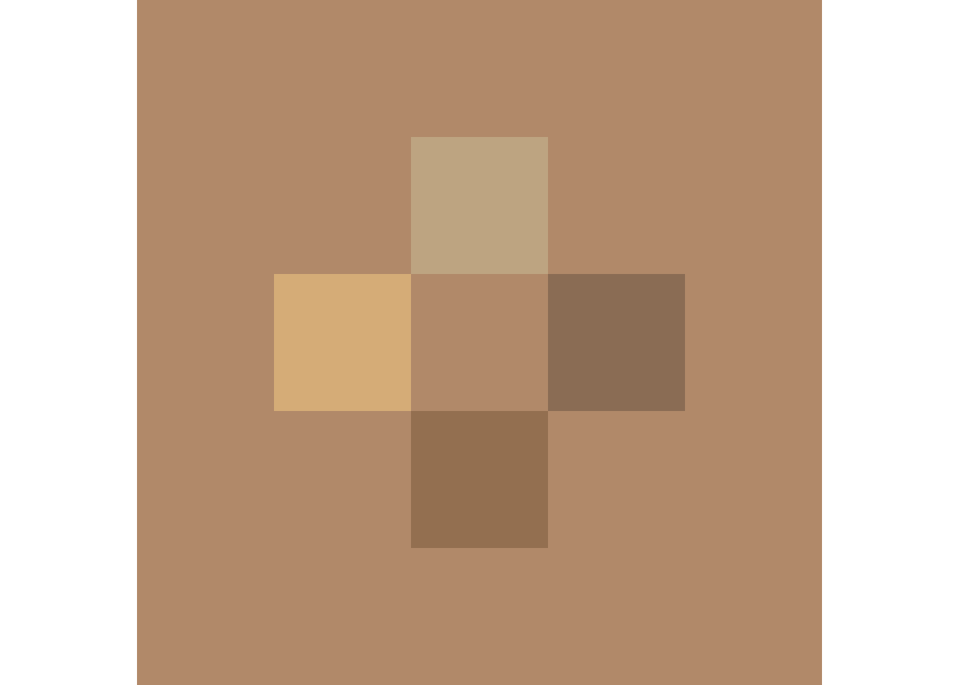

Note that the shading has given us a slight checkerboard pattern even though only one of the squares is elevated.

What happens if we render the same matrix as a three dimensional plot by calling plot_3d(elevation_matrix) function with the elevation matrix?

and render it using the plot_3d() method with the elevation matrix as an argument

simple_map %>%
  plot_3d(simple_matrix, linewidth=0)

rgl::rglwidget()

The zscale parameter to plot_3d() (with default zscale=1) allows us to scale the ratio of the x and y axis scales relative to the z axis. Reducing the zscale value has the effect of emphasising or magnifying the vertical z-dimension, whereas increasing the zscale value “flattens” the relief. For example, for x and y grid units of 1m, for a zscale of 2, 1m of elevation is rendered as elevation / zscale = height, to give 1 / 2 = 0.5m high).

12.3 The rayshader 3D Model Plinth

A solid base is applied to the model using the solid flag which has a default value of TRUE. The base thickness and colour are also controllable:

rgl::clear3d()

simple_map %>%
  plot_3d(simple_matrix,
          
          # Render base
          solid = TRUE,
          soliddepth = -0.50, #"auto" (= lowest_depth-1)
          solidcolor = "red",
          solidlinecolor = "blue",

        )

rgl::rglwidget()

We can remove the base by setting the solid parameter to plot_3d() to FALSE:

rgl::clear3d()

simple_map %>%
  plot_3d(simple_matrix,
          # Change the zscale
          zscale=2,
          # No base
          solid = FALSE
        )

r = rgl::rglwidget()
r

12.4 Saving the Widget as an HTML File

To save the HTML describing the WebGL model to a file for use elsewhere, we can use the htmlwidgets::saveWidget(widget, filename) function.

widget_fn = 'simple_3d_model.html'
htmlwidgets::saveWidget(r, widget_fn)

Embed the HTML back in an iframe:

htmltools::includeHTML(widget_fn)

If we save the html to a web location, we can then embed back the widget back as an external file loaded into an HTML iframe using knitr::include_url().

12.5 Rendering the Model to an Image File

#rgl::rgl.open()
#rgl::clear3d()
#mapped_route_yellow %>%
#  plot_3d(elmat, zscale = auto_zscale)

render_fn = "demo_model-1.png"

render_snapshot(render_fn)

#rgl::rgl.close()

knitr::include_graphics(render_fn)

12.6 Rendering High Quality Models

We can generate high quality renderings of a model using the rayshader::render_highquality() function:

library(rayrender)

# Open a connection to the renderer
#rgl::rgl.open()
rgl::clear3d()

simple_map %>%
  plot_3d(simple_matrix,
          # Change the zscale
          zscale=2,
          # No base
          solid = FALSE
        )

Sys.sleep(0.2)

hi_quality_fn = 'demo-hi-quality-matrix.png'

render_highquality(hi_quality_fn, samples=200,
                   scale_text_size = 24, clear=FALSE)

#Close connection
#rgl::rgl.close()

knitr::include_graphics(hi_quality_fn)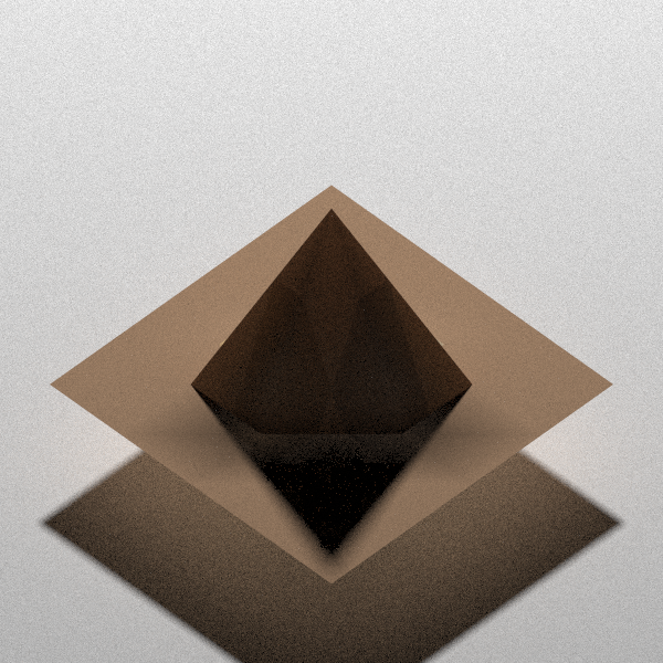

The high quality renderer provides a wide range of controls for composing the shot we want to render. For example one or more light sources can introduced, each with its own lightdirection, lightaltitude, lightsize, lightintensity and lightcolor setting. A range of camera controls in addition to controls provided by rgl window are also available, including camera_location and camera_lookat (a custom point at which the camera is directed). Experimenting with those settings will have to wait for another day!

For more discussion around rendering high quality images, see the rayshader: render_highquality#examples docs.

12.7 Making a 3D Print File

As well as visualising the map using an interactive 3D view, we can also export the model as a 3D printer ready model in the in the .stl file format using the rayshader::save_3dprint() function:

# Save the file to a 3d print stl file
#save_3dprint("stage_3d.stl", maxwidth = 10, unit = "in")

For another approach to generating 3D print model files from terrain data, see ChHarding/TouchTerrain_for_CAGEO /via @WRCStan.

12.8 Saving a Movie of a 3D Model

We can generate a movie file showing an animated view of the model using the rayshader::render_movie() function.

When operating in headless mode, movies are rendered using the webshot2 package. The launches a browser in the background which then renders the modelas a widget. This can be a slow process; rendering the following movie on my reasonably well-specced laptop took well over 10 minutes to render.

By default, we create a simple “turning model” movie, but the camera position, as well as lighting effects, can be scripted to allow us create the sort of scene we require. Who needs drone footage?!

# We need to load the av package to render the movie
library(av)

#options(rgl.useNULL = FALSE,
#        rgl.printRglwidget = FALSE)

# Open a connection to the renderer
rgl::rgl.open()

rgl::clear3d()
simple_map %>%
  plot_3d(simple_matrix)

# Render the movie to an MP4 file
video_fn = 'demo_3d_model.mp4'

#render_movie(video_fn)

rgl::rgl.close()

# Embed the movie
embedr::embed_video(video_fn, width = "256", height = "256")

The camera view used to generate the move can be configured according to several predefined paths using the rayshader::render_movie() path paramter and include the default orbit path, an oscillate path that covers a 90 degrees field of view and a custom path setting with which you can channel your inner principle photographer. Other parameters include the frame rate (fps) and the number of frames to render. A title bar can also be rendered.